...
- Command execution files
- problem_type_name.bat Operating system shell that executes the analysis process
")
Diagram depicting the files system (classic approach)
Appendix>'Classic' problemtype implementation>Implementation
Creating the Subdirectory for the Problem Type
Create the subdirectory "cmas2d.gid". This subdirectory has a .gid extension and will contain all the configuration files and calculating module files (.prb, .mat, .cnd, .bas, .bat, .exe).
NOTE: If you want the problem type to appear in the GiD Data->Problem type menu, create the subdirectory within "problemtypes", located in the GiD installation folder, for example C:\GiD\Problemtypes\cmas2d.gid
Appendix>'Classic' problemtype implementation>Implementation>Materials file
Create the materials file "cmas2d.mat". This file stores the physical properties of the material under study for the problem type. In this case, defining the density will be enough.
Enter the materials in the "cmas2d.mat" file using the following format:
MATERIAL: Name of the material (without spaces)
QUESTION: Property of the material. For this example, we are interested in the density of the material.
VALUE: Value of the property
HELP: A help text (optional field)
…
END MATERIAL
In GiD, the information in "cmas2d.mat" file is managed in the materials window, located in Data->Materials. 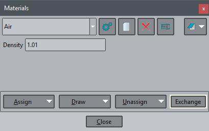
Materials window, for assigning materials to parts
MATERIAL: Air
QUESTION: Density
VALUE: 1.01
HELP: material density
END MATERIAL
MATERIAL: Steel
QUESTION: Density
VALUE: 7850
HELP: material density
END MATERIAL
MATERIAL: Aluminium
QUESTION: Density
VALUE: 2650
HELP: material density
END MATERIAL
Appendix>'Classic' problemtype implementation>Implementation>General file
Create the "cmas2d.prb" file. This file contains general information for the calculating module, such as the units system for the problem, or the type of resolution algorithm chosen.
Enter the parameters of the general conditions in "cmas2d.prb" using the following format:
PROBLEM DATA
QUESTION: Name of the parameter. If the name is followed by the #CB# instruction, the parameter is displayed as a combo box. The options in the menu must then be entered between parentheses and separated by commas.
For example, Unit_System#CB#(SI,CGS,User).
VALUE: The default value of the parameter.
…
END GENERAL DATA
In GiD, the information in the "cmas2d.prb" file is managed in the problem data window, which is located in Data->Problem Data. 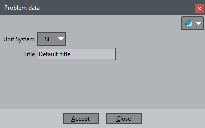
Problem Data window, to set general (non-spatial) data
PROBLEM DATA
QUESTION: Unit_System#CB#(SI,CGS,User)
VALUE: SI
QUESTION: Title
VALUE: Default_title
END GENERAL DATA
Appendix>'Classic' problemtype implementation>Implementation>Conditions file
Create the "cmas2d.cnd" file, which specifies the boundary and/or load conditions of the problem type in question. In the present case, this file is where the concentrated weights on specific points of the geometry are indicated.
Enter the boundary conditions using the following format:
CONDITION: Name of the condition
CONDTYPE: Type of entity which the condition is to be applied to. This includes the parameters "over points", "over lines", "over surfaces", "over volumes" or "over layers". In this example the condition is applied "over points".
CONDMESHTYPE: Type of entity of the mesh where the condition is to be applied. The possible parameters are "over nodes", "over body elements" or "over face elements". In this example, the condition is applied on nodes.
QUESTION: Name of the parameter of the condition
VALUE: Default value of the parameter
…
END CONDITION
…
In GiD, the information in the "cmas2d.cnd" file is managed in the conditions window, which is found in Data->Conditions.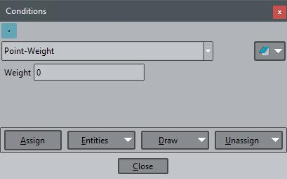
Conditions window, for assigning boundary conditions
CONDITION: Point-Weight
CONDTYPE: over points
CONDMESHTYPE: over nodes
QUESTION: Weight
VALUE: 0.0
HELP: Concentrated mass
END CONDITION
Appendix>'Classic' problemtype implementation>Implementation>Writing the calculation files
Create the "cmas2d.bas" file. This file will define the format of the .dat text file created by GiD. It will store the geometric and physical data of the problem. The .dat file will be the input to the calculating module.
NOTE: It is not necessary to have all the information registered in only one .bas file. Each .bas file has a corresponding .dat file.
Write the "cmas2d.bas" file as follows:
The format of the .bas file is based on commands. Text not preceded by an asterisk is reproduced exactly the same in the .dat file created by GiD. A text preceded by an asterisk is interpreted as a command.
Example:
.bas file
%%%% Problem Size %%%%
Number of Elements & Nodes:
*nelem *npoin
.dat file
%%%% Problem Size %%%%
Number of Elements & Nodes:
5379 4678
The contents of the "cmas2d.bas" file must be the following:
.bas file
...
==================================================================
General Data File
==================================================================
Title: *GenData(Title)
%%%%%%%%%%%%%%%%%% Problem Size %%%%%%%%%%%%%%%%%%%%%%%%%%%%%%%%%
Number of Elements & Nodes:
*nelem *npoin
In this first part of "cmas2d.bas" file, general information on the project is obtained.
*nelem: returns the total number of elements of the mesh.
*npoin: returns the total number of nodes of the mesh.
Coordinates: |
This command provides a rundown of all the nodes of the mesh, listing their identifiers and coordinates.
*loop, *end: commands used to indicate the beginning and the end of the loop. The command *loop receives a parameter.
*loop nodes: the loop iterates on nodes
*loop elems: the loop iterates on elements
*loop materials: the loop iterates on assigned materials
*format: the command to define the printing format. This command must be followed by a numerical format expressed in C syntax.
*NodesNum: returns the identifier of the present node
*NodesCoord: returns the coordinates of the present node
*NodesCoord (n, real): returns the x, y or z coordinate in terms of the value n:
n=1 returns the x coordinate
n=2 returns the y coordinate
n=3 returns the z coordinate
Connectivities: |
This provides a rundown of all the elements of the mesh and a list of their identifiers, the nodes that form them, and their assigned material.
*set elems(all): the command to include all element types of the mesh when making the loop.
*ElemsNum: returns the identifier of the present element
*ElemsConec: returns the nodes of an element in a counterclockwise order
*ElemsMat: returns the number of the assigned material of the present element
Begin Materials |
This gives the total number of materials in the project
*nmats: returns the total number of materials
...
This provides a rundown of all the materials in the project and a list of the identifiers and densities for each one.
*MatProp (density, real): returns the value of the property "density" of the material in a "real" format.
*Operation (expression): returns the result of an arithmetic expression. This operation must be expressed in C.
*Set var PROP1(real)=Operation(MatProp(Density, real)): assigns the value returned by MatProp (which is the value of the density of the material) to the variable PROP1 (a "real" variable).
*PROP1: returns the value of the variable PROP1.
*MatNum: returns the identifier of the present material.
...
This provides the number of entities with a particular condition.
*Set Cond Point-Weight *nodes: this command enables you to select the condition to work with from that moment on. For the present example, select the condition "Point-Weight".
*CondNumEntities(int): returns the number of entities with a certain condition.
*Set var NFIX(int)= CondNumEntities(int): assigns the value returned by the command CondNumEntities to the NFIX variable (an "int" variable).
*NFIX: returns the value of the NFIX variable.
...
This provides a rundown of all the nodes with the condition "Point-Weight" with a list of their identifiers and the first "weight" field of the condition in each case.
*loop nodes *OnlyInCond: executes a loop that will provide a rundown of only the nodes with this condition.
*cond(1): returns the number 1 field of a condition previously selected with the *set cond command. The field of the condition may also be selected using the name of the condition, for example cond(weight).
cmas2d.bas
==================================================================
General Data File
==================================================================
%%%%%%%%%%%%%%%%%% Problem Size %%%%%%%%%%%%%%%%%%%%%%%%%%%%%%%%%
Number of Elements & Nodes:
*nelem *npoin
%%%%%%%%%%%%%%%%%%% Mesh Database %%%%%%%%%%%%%%%%%%%%%%%%%%%%%%%
Coordinates:
Node X Y
*set elems(all)
*loop nodes
*format "%5i%14.5e%14.5e"
*NodesNum *NodesCoord(1,real) *NodesCoord(2,real)
*end nodes
.................................................................
Connectivities:
Element Node(1) Node(2) Node(3) Material
*loop elems
*format "%10i%10i%10i%10i%10i"
*ElemsNum *ElemsConec *ElemsMat
*end elems
.................................................................
Begin Materials
Nº Materials= *nmats
Mat. Density
.................................................................
*loop materials
*format "%4i%13.5e"
*set var PROP1(real)=Operation(MatProp(Density, real))
*MatNum *PROP1
*end
.................................................................
Point conditions
*Set Cond Point-Weight *nodes
*set var NFIX(int)=CondNumEntities(int)
Concentrated Weights
*NFIX
.................................................................
Potentials Prescrits:
Node Tipus
Valor/Etiqueta
*Set Cond Point-Weight *nodes
*loop nodes *OnlyInCond
*NodesNum *cond(1)
*end
.................................................................
Appendix>'Classic' problemtype implementation>Implementation>Solver
Create the file "cmas2d.c". This file contains the code for the execution program of the calculating module. This execution program reads the problem data provided by GiD, calculates the coordinates of the center of mass of the object and the distance between each element and this point. These results are saved in a text file with the extension .post.res.
Compile and link the "cmas2d.c" file in order to obtain the executable cmas2d.exe file.
The calculating module (cmas2d.exe) reads and generates the files described below.
...
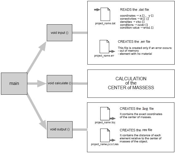
cmas2d.c solver structure
NOTE: The "cmas2d.c" code is explained in the appendix.
Appendix>'Classic' problemtype implementation>Implementation>Run the solver
Create the "cmas2d.win.bat" file. This file connects the data file(s) (.dat) to the calculating module (the cmas2d.exe program). When the GiD Calculate option is selected, it executes the .bat file for the problem type selected.
When GiD executes the .bat file, it transfers three parameters in the following way:
(parameter 3) / *.bat (parameter 2) / (parameter 1)
parameter 1: project name
parameter 2: project directory
parameter 3: Problem type location directory
NOTE: The .win.bat fiile as used in Windows is explained below; the shell script for UNIX systems is also included with the documentation of this tutorial.
rem OutputFile: %2%1.log |
...
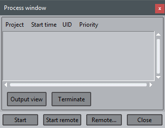
The process window
...
rem ErrorFile: %2%1.err
A comment line such as "rem ErrorFile: file_name.err" means that the indicated file will contain the errors (if any). If the .err file is present at the end of the execution, a window comes up showing the error. The absence of the .err file indicates that the calculation is considered satisfactory.
GiD automatically deletes the .err files before initiating a calculation to avoid confusion.
del %2%1.log |
This deletes results files from any previous calculations to avoid confusion.
%3\cmas2d.exe %2%1 |
This executing the cmas2d.exe and provide the .dat as input file file.
Appendix>'Classic' problemtype implementation>Using the problemtype with an example
In order to understand the way the calculating module works, simple problems with limited practical use have been chosen. Although these problems do not exemplify the full potential of the GiD program, the user may intuit their answers and, therefore, compare the predicted results with those obtained in the simulations.
- . Create a surface, for example from the menu Geometry->Create->Object->Polygon
- . Create a polygon with 5 sides, centered in the (0,0,0) and located in the XY plane (normal = 0,0,1) and whit radius=1.0
...
- . Load the problemtype: menu Data->Problem type->cmas2d.
- . Choose Data->Materials.
- . The materials window is opened. From the Materials menu in this window, choose the option Air.
...
- . Click Assign->Surfaces and select the surface. Press <Esc> when this step is finished.
- . Choose the Data->Conditions option. A window is opened in which the conditions of the problem should be entered.
...
- . Enter the value 1e3 in the Weight box. Click Assign and select the upper corner point. Press <Esc> when this step is finished.
- . Choose the Mesh->Generate option.
- . A window appears in which to enter the maximum element size for the mesh to be generated. Accept the default value and click OK. The mesh shown will be obtained.
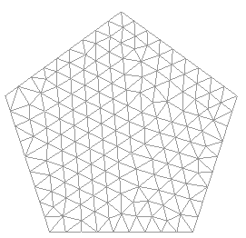
The mesh of the object
- . Now the calculation may be initiated, but first the model must be saved (Files->Save), use 'example_cmas2d' as name for the model.
- . Choose the Calculate option from the Calculate menu to start the calculation module.
- . Wait until a box appears indicating the calculation has finished.
...
- . Select the option Files->Postprocess.
- . Select Window->View results.
- . A window appears from which to visualize the results. By default when changing to postprocesses mode no results is visualized.
- . From the View combo box in the View Results window, choose the Contour Fill option. A set of available results (only one for this case) are displayed.
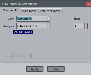
- . Now choose the MC-DISTANCE result and click Apply. A graphic representation of the calculation is obtained.
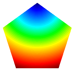
Visualizing the distance from the weighted center of mass to each point
The results shown on the screen reproduce those we anticipated at the outset of the problem: the center of mass of an object is not in its geometric center because a concentrated mass on the top. The .log file will provide the exact coordinates of the calculated mass center.