Once you have generated the mesh, and assigned the conditions and the materials properties, as well as the general problem and intervals data for the solver, it is necessary to produce the data input files to be processed by that program.
To manage this reading, GiD is able to interpret a file called problem_type_name.bas (where problem_type_name is the name of the working directory of the problem type without the .bas extension).
This file (template file) describes the format and structure of the required data input file for the solver that is used for a particular case. This file must remain in the problem_type_name.gid directory, as well as the other files already described - problem_type_name.cnd, problem_type_name.mat, problem_type_name.prb and also problem_type_name.sim and ***.geo, if desired.
In the case that more than one data input file is needed, GiD allows the creation of more files by means of additional ***.bas files (note that while problem_type_name.bas creates a data input file named project_name.dat, successive ***.bas files - where *** can be any name - create files with the names project_name-1.dat, project_name-2.dat, and so on). The new files follow the same rules as the ones explained next for problem_type_name.bas files.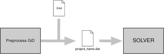
These files work as an interface from GiD's standard results to the specific data input for any individual solver module. This means that the process of running the analysis simply forms another step that can be completed within the system.
In the event of an error in the preparation of the data input files, the programmer has only to fix the corresponding problem_type_name.bas or ***.bas file and rerun the example, without needing to leave GiD, recompile or reassign any data or re-mesh.
This facility is due to the structure of the template files. They are a group of macros (like an ordinary programming language) that can be read, without the need of a compiler, every time the corresponding analysis file is to be written. This ensures a fast way to debug mistakes.
PROBLEMTYPE 'CLASSIC'>Template files>Commands used in the .bas file
List of bas commands: (all these commands must be prefixed by a character *)
Add
Break
Clock Cond CondElemFace CondHasLocalAxes CondName CondNumEntities CondNumFields
ElemsCenter ElemsConec ElemsLayerName ElemsLayerNum ElemsMat ElemsMatProp ElemsNnode ElemsNnodeCurt ElemsNNodeFace ElemsNNodeFaceCurt ElemsNormal ElemsNum ElemsRadius ElemsType ElemsTypeName Else ElseIf End Endif
FaceElemsNum FaceIndex FactorUnit FileId For Format
GenData GlobalNodes GroupColorRGB GroupFullName GroupName GroupNum GroupNumEntities GroupParentName GroupParentNum
If Include IntFormat IntvData IsQuadratic
LayerColorRGB LayerName LayerNum LayerNumEntities LocalAxesDef LocalAxesDefCenter LocalAxesNum LocalNodes Loop LoopVar
MaterialLocalNum MatNum MatProp MessageBox
Ndime Nelem Nintervals NLocalAxes Nmats Nnode NodesCoord NodesLayerName NodesLayerNum NodesNum Npoin
Operation
RealFormat Remove
Set SetFormatForceWidth SetFormatStandard
Tcl Time
Units
WarningBox
PROBLEMTYPE 'CLASSIC'>Template files>Commands used in the .bas file>Single value return commands
When writing a command, it is generally not case-sensitive (unless explicitly mentioned), and even a mixture of uppercase and lowercase will not affect the results.
- *npoin, *ndime, *nnode, *nelem, *nmats, *nintervals. These return, respectively, the number of points, the dimensions of the project being considered, the number of nodes of the element with the highest number, the number of elements, the number of materials and the number of data intervals. All of them are considered as integers and do not carry arguments (see *format,*intformat), except *nelem, which can bring different types of elements. These elements are: Point, Linear, Triangle, Quadrilateral, Tetrahedra, Hexahedra, Prism, Pyramid, Sphere, depending on the number of edges the element has, and All, which comprises all the possible types. The command *nmats returns the number of materials effectively assigned to an entity, not all the defined ones.
- *GenData. This must carry an argument of integer type that specifies the number of the field to be printed. This number is the order of the field inside the general data list. This must be one of the values that are fixed for the whole problem, independently of the interval (see Problem and intervals data file (.prb)). The name of the field, or an abreviation of it, can also be the argument instead. The arguments REAL or INT, to express the type of number for the field, are also available (see *format,*intformat,*realformat,*if). If they are not specified, the program will print a character string. It is mandatory to write one of them within an expression, except for strcmp and strcasecmp. The numeration must start with the number 1.
Note: Using this command without any argument will print all fields
- *IntvData. The only difference between this and the previous command is that the field must be one of those fields varying with the interval (see Problem and intervals data file (.prb)). This command must be within a loop over intervals (see *loop) and the program will automatically update the suitable value for each iteration.
Note: Using this command without any argument will print all fields
- *MatProp. This is the same as the previous command except that it must be within a loop over the materials (see *loop). It returns the property whose field number or name is defined by its argument. It is recommended to use names instead of field numbers.
If the argument is 0, it returns the material's name.
Note: Using this command without any argument will print all fields
Caution: If there are materials with different numbers of fields, you must ensure not to print non-existent fields using conditionals.
- MaterialLocalNum To get the local material number from its global id or its name.
The local material id is the material number for the calculation file, taking into account the materials applied to mesh elements)
It has a single argument, an integer of the material global number or its name.
Example:
*set var i_material=3
*MaterialLocalNum(*i_material)
*MaterialLocalNum(Steel)
- *ElemsMatProp. This is the same as Matprop but uses the material of the current element. It must be within a loop over the elements (see *loop). It returns the property whose field number or name is defined by its argument. It is recommended to use names instead of field numbers.
Example:
*loop elements
*elemsnum *elemsmat *elemsmatprop(young)
*end elements
- *Cond. The same remarks apply here, although now you have to notify with the command *set (see *set) which is the condition being processed. It can be within a loop (see *loop) over the different intervals should the conditions vary for each interval.
Note: Using this command without any argument will print all fields
- *CondName. This returns the conditions's name. It must be used in a loop over conditions or after a *set cond command.
- *CondNumFields. This returns the number of fields of the current condition. It must be used in a loop over conditions or after *set cond
- *CondHasLocalAxes. returns 1 if the condition has a local axis field, 0 else
- *CondNumEntities. You must have previously selected a condition (see *set cond). This returns the number of entities that have a condition assigned over them.
- *ElemsNum: This returns the element's number.
*NodesNum: This returns the node's number.
*MatNum: This returns the material's number.
*ElemsMat: This returns the number of the material assigned to the element.
All of these commands must be within a proper loop (see *loop) and change automatically for each iteration. They are considered as integers and cannot carry any argument. The number of materials will be reordered numerically, beginning with number 1 and increasing up to the number of materials assigned to any entity.
- *FaceElemsNum: must be inside a *loop faces, and print the element's number owner of the face
- *FaceIndex: must be inside a *loop faces, and print the face index on the element (starting from 1)
- *LayerNum: This returns the layer's number.
*LayerName: This returns the layer's name.
*LayerColorRGB: This returns the layer's color in RGB (three integer numbers between 0 and 256). If parameter (1), (2) or (3) is specified, the command returns only the value of one color. RED is 1, GREEN is 2 and BLUE is 3.
The commands *LayerName, *LayerNum and *LayerColorRGB must be inside a loop over layers; you cannot use these commands in a loop over nodes or elements.
Example:
*loop layers
*LayerName *LayerColorRGB
*Operation(LayerColorRGB(1)/255.0) *Operation(LayerColorRGB(2)/255.0) *Operation(LayerColorRGB(3)/255.0)
*end layers
- *NodesLayerNum: This returns the layer's number. It must be used in a loop over nodes.
*NodesLayerName: This returns the layer's name. It must be used in a loop over nodes.
*ElemsLayerNum: This returns the layer's number. It must be used in a loop over elems.
*ElemsLayerName: This returns the layer's name. It must be used in a loop over elems.
- *LayerNumEntities. You must have previously selected a layer (see *set layer). This returns the number of entities that are inside this layer.
- *GroupNum: This returns the group's index number.
*GroupFullName: This returns the full group's name, including parents separed by //. e.g: a//b//c
*GroupName: This returns only the tail group's name. e.g: c (if group's doesn't has parent then is the same as the full name)
*GroupColorRGB: This returns the group's color in RGB (three integer numbers between 0 and 256). If parameter (1), (2) or (3) is specified, the command returns only the value of one color. RED is 1, GREEN is 2 and BLUE is 3.
*GroupParentName: This returns the name of the parent of the current group
*GroupParentNum: This returns the index of the parent of the current group
These commands must be inside a loop over groups, or after set group.
Example:
*loop groups
*groupnum "*GroupFullName" ("*groupname" parent:*groupparentnum) *groupcolorrgb
*set group *GroupName *nodes
*if(GroupNumEntities)
nodes: *GroupNumEntities
*loop nodes *onlyingroup
*nodesnum
*end nodes
*end if
*set group *GroupName *elems
*if(GroupNumEntities)
elements: *GroupNumEntities
*loop elems *onlyingroup
*elemsnum
*end elems
*end if
*set group *GroupName *faces
*if(GroupNumEntities)
faces: *GroupNumEntities
*loop faces *onlyingroup
*faceelemsnum:*faceindex
*end faces
*end if
*end groups
- *GroupNumEntities. You must have previously selected a group (see *set group). This returns the number of entities that are inside this group.
- *LoopVar. This command must be inside a loop and it returns, as an integer, what is considered to be the internal variable of the loop. This variable takes the value 1 in the first iteration and increases by one unit for each new iteration. The parameter elems,nodes,materials,intervals, used as an argument for the corresponding loop, allows the program to know which one is being processed. Otherwise, if there are nested loops, the program takes the value of the inner loop.
- *Operation. This returns the result of an arithmetical expression what should be written inside parentheses immediately after the command. This operation must be defined in C-format and can contain any of the commands that return one single value. You can force an integer or a real number to be returned by means of the parameters INT or REAL. Otherwise, GiD returns the type according to the result.
The valid C-functions that can be used are:
- +,-,*,/,%,(,),=,<,>,!,&,|, numbers and variables
- sin
- cos
- tan
- asin
- acos
- atan
- atan2
- exp
- fabs
- abs
- pow
- sqrt
- log
- log10
- max
- min
- strcmp
- strcasecmp
The following are valid examples of operations:
*operation(4*elemsnum+1)
operation(8(loopvar-1)+1)
Note: There cannot be blank spaces between the commands and the parentheses that include the parameters.
Note: Commands inside *operation do not need * at the beginning.
- *LocalAxesNum. This returns the identification name of the local axes system, either when the loop is over the nodes or when it is over the elements, under a referenced condition.
- *nlocalaxes. This returns the number of the defined local axes system.
- *IsQuadratic. This returns the value 1 when the elements are quadratic or 0 when they are not.
- *Time. This returns the number of seconds elapsed since midnight.
- *Clock. This returns the number of clock ticks (aprox. milliseconds) of elapsed processor time.
Example:
*set var t0=clock
*loop nodes
*nodescoord
*end nodes
*set var t1=clock
ellapsed time=*operation((t1-t0)/1000.0) seconds
- *Units('magnitude'). This returns the current unit name for the selected magnitude (the current unit is the unit shown inside the unit window).
Example:
*Units(LENGTH)
- *FactorUnit('unit'). This returns the numeric factor to convert a magnitude from the selected unit to the basic unit.
Example:
*FactorUnit(PRESSURE)
- *FileId returns a long integer representing the calculaton file, written following the current template.
This value must be used to provide the channel of the calculation file to a tcl procedure to directly print data with the GiD_File fprintf special Tcl command.
PROBLEMTYPE 'CLASSIC'>Template files>Commands used in the .bas file>Multiple values return commands
These commands return more than one value in a prescribed order, writing them one after the other. All of them except LocalAxesDef are able to return one single value when a numerical argument giving the order of the value is added to the command. In this way, these commands can appear within an expression. Neither LocalAxesDef nor the rest of the commands without the numerical argument can be used inside expressions. Below, a list of the commands with the appropriate description is displayed.
- *NodesCoord. This command writes the node's coordinates. It must be inside a loop (see *loop) over the nodes or elements. The coordinates are considered as real numbers (see *realformat and *format). It will write two or three coordinates according to the number of dimensions the problem has (see *Ndime).
If *NodesCoord receives an integer argument (from 1 to 3) inside a loop of nodes, this argument indicates which coordinate must be written: x, y or z. Inside a loop of nodes:
*NodesCoord writes three or two coordinates depending on how many dimensions there are.
NodesCoord(1) writes the *x coordinate of the actual node of the loop.
NodesCoord(2) writes the *y coordinate of the actual node of the loop.
NodesCoord(3) writes the *z coordinate of the actual node of the loop.
If the argument real is given, the coordinates will be treated as real numbers.
Example: using *NodesCoord inside a loop of nodes
Coordinates:
Node X Y
*loop nodes
*format "%5i%14.5e%14.5e"
*NodesNum *NodesCoord(1,real) *NodesCoord(2,real)
*end nodes
This command effects a rundown of all the nodes in the mesh, listing their identifiers and coordinates (x and y).
The contents of the project_name.dat file could be something like this:
Coordinates:
Node X Y
1 -1.28571e+001 -1.92931e+000
2 -1.15611e+001 -2.13549e+000
3 -1.26436e+001 -5.44919e-001
4 -1.06161e+001 -1.08545e+000
5 -1.12029e+001 9.22373e-002
...
*NodesCoord can also be used inside a loop of elements. In this case, it needs an additional argument that gives the local number of the node inside the element. After this argument it is also possible to give which coordinate has to be written: x, y or z.
Inside a loop of elements:
*NodesCoord(4) writes the coordinates of the 4th node of the actual element of the loop.
NodesCoord(5,1) writes the *x coordinate of the 5th node of the actual element of the loop.
NodesCoord(5,2) writes the *y coordinate of the 5th node of the actual element of the loop.
NodesCoord(5,3) writes the *z coordinate of the 5th node of the actual element of the loop.
- *ElemsConec. This command writes the element's connectivities, i.e. the list of the nodes that belong to the element, displaying the direction for each case (anti-clockwise direction in 2D, and depending on the standards in 3D). For shells, the direction must be defined. However, this command accepts the argument swap and this implies that the ordering of the nodes in quadratic elements will be consecutive instead of hierarchical. The connectivities are considered as integers (see *intformat and *format).
If *ElemsConec receives an integer argument (begining from 1), this argument indicates which element connectity must be written:
*loop elems
all conectivities: *elemsconec
first conectivity *elemsconec(1)
*end elems
Note: In the first versions of GiD, the optional parameter of the last command explained was invert instead of swap, as it is now. It was changed due to technical reasons. If you have an old .bas file prior to this specification, which contains this command in its previous form, when you try to export the calculation file, you will be warned about this change of use. Be aware that the output file will not be created as you expect.
- *GlobalNodes. This command returns the nodes that belong to an element's face where a condition has been defined (on the loop over the elements). The direction for this is the same as for that of the element's connectivities. The returned values are considered as integers (see *intformat and *format).If *GlobalNodes receives an integer argument (beginning from 1), this argument indicates which face connectity must be written.
So, the local numeration of the faces is:
Triangle: 1-2 2-3 3-1
Quadrilateral: 1-2 2-3 3-4 4-1
Tetrahedra: 1-2-3 2-4-3 3-4-1 4-2-1
Hexahedra: 1-2-3-4 1-4-8-5 1-5-6-2 2-6-7-3 3-7-8-4 5-8-7-6
Prism: 1-2-3 1-4-5-2 2-5-6-3 3-6-4-1 4-5-6
Pyramid: 1-2-3-4 1-5-2 2-5-3 3-5-4 4-5-1
- *LocalNodes. The only difference between this and the previous one is that the returned value is the local node's numbering for the corresponding element (between 1 and nnode).
- *CondElemFace. This command return the number of face of the element where a condition has been defined (beginning from 1). The information is equivalent to the obtained with the localnodes command
- *ElemsNnode. This command returns the number of nodes of the current element (valid only inside a loop over elements).
Example:
*loop elems
*ElemsNnode
*end elems
- *ElemsNnodeCurt. This command returns the number of vertex nodes of the current element (valid only inside a loop over elements). For example, for a quadrilateral of 4, 8 or 9 nodes, it returns the value 4.
- *ElemsNNodeFace. This command returns the number of face nodes of the current element face (valid only inside a loop over elements onlyincond, with a previous *set cond of a condition defined over face elements).
Example:
*loop elems
*ElemsNnodeFace
*end elems
- *ElemsNNodeFaceCurt. This command returns the short (corner nodes only) number of face nodes of the current element face (valid only inside a loop over elements onlyincond, with a previous *set cond of a condition defined over face elements).
Example:
*loop elems
*ElemsNnodeFaceCurt
*end elems
- *ElemsType: This returns the current element type as a integer value: 1=Linear, 2=Triangle, 3=Quadrilateral, 4=Tetrahedra, 5=Hexahedra, 6=Prism, 7=Point,8=Pyramid,9=Sphere,10=Circle. (Valid only inside a loop over elements.)
- *ElemsTypeName: This returns the current element type as a string value: Linear, Triangle, Quadrilateral, Tetrahedra, Hexahedra, Prism, Point, Pyramid, Sphere, Circle. (Valid only inside a loop over elements.)
- *ElemsCenter: This returns the element center. (Valid only inside a loop over elements.)
Note: This command is only available in GiD version 9 or later.
- *ElemsRadius: This returns the element radius. (Valid only inside a loop over sphere or Circle elements.)
Note: This command is only available in GiD version 8.1.1b or later.
- *ElemsNormal. This command writes the normal's coordinates. It must be inside a loop (see *loop) over elements, and it is only defined for triangles, quadrilaterals, and circles (and also for lines in 2D cases).
If *ElemsNormal receives an integer argument (from 1 to 3) this argument indicates which coordinate of the normal must be written: x, y or z.
- *LocalAxesDef. This command returns the nine numbers that define the transformation matrix of a vector from the local axes system to the global one.
Example:
*loop localaxes
*format "%10.4lg %10.4lg %10.4lg"
x'=*LocalAxesDef(1) *LocalAxesDef(4) *LocalAxesDef(7)
*format "%10.4lg %10.4lg %10.4lg"
y'=*LocalAxesDef(2) *LocalAxesDef(5) *LocalAxesDef(8)
*format "%10.4lg %10.4lg %10.4lg"
z'=*LocalAxesDef(3) *LocalAxesDef(6) *LocalAxesDef(9)
*end localaxes
- *LocalAxesDef(EulerAngles). This is as the last command, only with the EulerAngles option. It returns three numbers that are the 3 Euler angles (radians) that define a local axes system

![]()
Rotation of a vector expressed in terms of euler angles.
How to calculate X[3] Y[3] Z[3] orthonormal vector axes from three euler angles angles[3]
X[0]= cosC*cosA - sinC*cosB*sinA
X[1]= -sinC*cosA - cosC*cosB*sinA
X[2]= sinB*sinA
Y[0]= cosC*sinA + sinC*cosB*cosA
Y[1]= -sinC*sinA + cosC*cosB*cosA
Y[2]= -sinB*cosA
Z[0]= sinC*sinB
Z[1]= cosC*sinB
Z[2]= cosB
where
cosA=cos(angles[0])
sinA=sin(angles[0])
cosB=cos(angles[1])
sinB=sin(angles[1])
cosC=cos(angles[2])
sinC=sin(angles[2])
How to calculate euler angles angles[3] from X[3] Y[3] Z[3] orthonormal vector axes
if(Z[2]<1.0-EPSILON && Z[2]>-1.0+EPSILON){
double senb=sqrt(1.0-Z[2]*Z[2]);
angles[1]=acos(Z[2]);
angles[2]=acos(Z[1]/senb);
if(Z[0]/senb<0.0) angles[2]=M_2PI-angles[2];
angles[0]=acos(-Y[2]/senb);
if(X[2]/senb<0.0) angles[0]=M_2PI-angles[0];
} else {
angles[1]=acos(Z[2]);
angles[0]=0.0;
angles[2]=acos(X[0]);
if(-X[1]<0.0) angles[2]=M_2PI-angles[2];
}
- *LocalAxesDefCenter. This command returns the origin of coordinates of the local axes as defined by the user. The "Automatic" local axes do not have a center, so the point (0,0,0) is returned. The index of the coordinate (from 1 to 3) can optionally be given to LocalAxesDefCenter to get the x, y or z value.
Example:
*LocalAxesDefCenter
*LocalAxesDefCenter(1) *LocalAxesDefCenter(2) *LocalAxesDefCenter(3)
PROBLEMTYPE 'CLASSIC'>Template files>Commands used in the .bas file>Specific commands
** To avoid line-feeding you need to write **{}, so that the line currently being used continues on the following line of the file filename.bas.
- *# If this is placed at the beginning of the line, it is considered as a comment and therefore is not written.
- **** In order for an asterisk symbol to appear in the text, two asterisks **** must be written.
- *Include. The include command allows you to include the contents of a slave file inside a master .bas file, setting a relative path from the Problem Type directory to this secondary file.
Example:
*include includes\execntrlmi.h
Note: The *.bas extension cannot be used for the slave file to avoid multiple output files.
- *MessageBox. This command stops the execution of the .bas file and prints a message in a window; this command should only be used when a fatal error occurs.
Example:
*MessageBox error: Quadrilateral elements are not permitted.
- *WarningBox. This is the same as MessageBox, but the execution is not stopped.
Example:
WarningBox Warning: Exist Bad elements. A STL file is a collection of triangles bounding a volume.
The following commands must be written at the beginning of a line and the rest of the line will serve as their modifiers. No additional text should be written.
- *loop, *end, *break. These are declared for the use of loops. A loop begins with a line that starts with loop (none of these commands is case-sensitive) and contains another word to express the variable of the loop. There are some lines in the middle that will be repeated depending on the values of the variable, and whose parameters will keep on changing throughout the iterations if necessary. Finally, a loop will end with a line that finishes with *end. After *end, you may write any kind of comments in the same line. The command **break inside a *loop or *for block, will finish the execution of the loop and will continue after the *end line.
The variables that are available for *loop are the following:
- elems, nodes, faces, materials, conditions, layers, groups, intervals, localaxes. These commands mean, respectively, that the loop will iterate over the elements, nodes, faces of a group, materials, conditions, layers, groups, intervals or local axes systems. The loops can be nested among them. The loop over the materials will iterate only over the effectively assigned materials to an entity, in spite of the fact that more materials have been defined. The number of the materials will begin with the number 1. If a command that depends on the loop is located outside it, the number will also take by default the value 1.
After the command *loop:
- If the variable is nodes, elems or faces, you can include one of the modifiers: *all, *OnlyInCond,*OnlyInLayer or *OnlyInGroup. The first one signifies that the iteration is going to be performed over all the entities.
The *OnlyInCond modifier implies that the iteration will only take place over the entities that satisfy the relevant condition. This condition must have been previously defined with *set cond.
*OnlyInLayer implies that the iteration will only take place over the entities that are in the specified layer; layers must be specified with the command *set Layer.
*OnlyInGroup implies that the iteration will only take place over the entities that are in the specified group;
group must be specified inside a loop groups with the command *set Group *GroupName *nodes|elems|faces, or *set Group <name> , with <name> the full name of the group.
By default, it is assumed that the iteration will affect all the entities. - If the variable is material you can include the modifier *NotUsed to make a loop over those materials that are defined but not used.
- If the variable is conditions you must include one of the modifiers: *Nodes, *BodyElements, *FaceElements, *Layers or *Groups, to do the loop on the conditions defined over this kind of mesh entity, or only the conditions declared 'over layers' or only the ones declared 'over groups'.
- If the variable is layers you can include modifiers: OnlyInCond if before was set a condition defined 'over layers'
- If the variable is groups you can include modifiers: OnlyInCond if before was set a condition defined 'over groups' (e.g. inside a *loop conditions *groups)
Example 1:
*loop nodes
*format "%5i%14.5e%14.5e"
*NodesNum *NodesCoord(1,real) *NodesCoord(2,real)
*end nodes
This command carries out a rundown of all the nodes of the mesh, listing their identifiers and coordinates (x and y coordinates).
Example 2:
*Set Cond Point-Weight *nodes
*loop nodes OnlyInCond
*NodesNum *cond(1)
*end
This carries out a rundown of all the nodes assigned the condition "Point-Weight" and provides a list of their identifiers and the first "weight" field of the condition in each case.
Example 3:
*Loop Elems
*ElemsNum *ElemsLayerNum
*End Elems
This carries out a rundown of all the elements and provides a list of their identifier and the identifier of the layer to which they belong.
Example 4:
*Loop Layers
*LayerNum *LayerName *LayerColorRGB
*End Layers
This carries out a rundown of all the layers and for each layer it lists its identifier and name.
Example 5:
*Loop Conditions OverFaceElements
*CondName
*Loop Elems OnlyInCond
*elemsnum *condelemface *cond
*End Elems
*End Conditions
This carries out a rundown of all conditions defined to be applied on the mesh 'over face elements', and for each condition it lists its name and for each element where this condition is applied are printed the element number, the marked face and the condition field values.
Example 6:
*loop intervals
interval=*loopvar
*loop conditions *groups
*if(condnumentities)
condition name=*condname
*loop groups *onlyincond
*groupnum *groupname *cond
*end groups
*end if
*end conditions
*end intervals
This do a loop for each interval, and for each condition defined 'over groups' list the groups where the condition was applied and its values.
- *if, *else, *elseif, *endif. These commands create the conditionals. The format is a line which begins with *if followed by an expression between parenthesis. This expression will be written in C-language syntax, value return commands, will not begin with *, and its variables must be defined as integers or real numbers (see *format, *intformat, *realformat), with the exception of strcmp and strcasecmp. It can include relational as well as arithmetic operators inside the expressions.
The following are valid examples of the use of the conditionals:
*if((fabs(loopvar)/4)<1.e+2)
*if((p3<p2)||p4)
*if((strcasecmp(cond(1),"XLoad")==0)&&(cond(2)!=0))
The first example is a numerical example where the condition is satisfied for the values of the loop under 400, while the other two are logical operators; in the first of these two, the condition is satisfied when p3<p2 or p4 is different from 0, and in the second, when the first field of the condition is called XLoad (with this particular writing) and the second is not null.
If the checked condition is true, GiD will write all the lines until it finds the corresponding *else, *elseif or *endif (*end is equivalent to *endif after *if). *else or *elseif are optional and require the writing of all the lines until the corresponding *endif, but only when the condition given by *if is false. If either *else or *elseif is present, it must be written between *if and *endif. The conditionals can be nested among them.
The behaviour of *elseif is identical to the behaviour of *else with the addition of a new condition:
*if(GenData(31,int)==1)
...(1)
*elseif(GenData(31,int)==2)
...(2)
*else
...(3)
*endif
In the previous example, the body of the first condition (written as 1) will be written to the data file if GenData(31,int) is 1, the body of the second condition (written as 2) will be written to the data file if GenData(31,int) is 2, and if neither of these is true, the body of the third condition (written as 3) will be written to the data file.Note: A conditional can also be written in the middle of a line. To do this, begin another line and write the conditional by means of the command *{}.
- *for, *end, *break. The syntax of this command is equivalent to *for in C-language.
*for(varname=expr.1;varname<=expr.2;varname=varname+1)
*end for
The meaning of this statement is the execution of a controlled loop, since varname is equal to expr.1 until it is equal to expr.2, with the value increasing by 1 for each step. varname is any name and expr.1 and expr.2 are arithmetical expressions or numbers whose only restrictions are to express the range of the loop.
The command *break inside a *loop or *for block, will finish the execution of the loop and will continue after the *end line.
Example:
*for(i=1;i<=5;i=i+1)
variable i=*i
*end for
- *set. This command has the following purposes:
- *set cond: To set a condition.
- *set Layer "layer name" *nodes|elems: To set a layer.
- *set Group "group name" *nodes|elems|faces: To set a group. (inside a *loop groups can use *GroupName as "group name" ,to get the name of the group of the current loop)
- *set elems: To indicate the elements.
- *set var: To indicate the variables to use.
It is not necessary to write these commands in lowercase, so *Set will also be valid in all the examples.
*set cond.: In the case of the conditions, GiD allows the combination of a group of them via the use of *add cond. When a specific condition is about to be used, it must first be defined, and then this definition will be used until another is defined. If this feature is performed inside a loop over intervals, the corresponding entities will be chosen. Otherwise, the entities will be those referred to in the first interval.
It is done in this way because when you indicate to the program that a condition is going to be used, GiD creates a table that lets you know the number of entities over which this condition has been applied. It is necessary to specify whether the condition takes place over the *nodes, over the *elems or over *layers to create the table.
So, a first example to check the nodes where displacement constraints exist could be:
*Set Cond Volu-Cstrt *nodes
*Add Cond Surf-Cstrt *nodes
*Add Cond Line-Cstrt *nodes
*Add Cond Poin-Cstrt *nodes
These let you apply the conditions directly over any geometric entity.
*Set Layer "layer name" *elems|nodes
*Add Layer "layer name"
*Remove Layer "layer name"
This command sets a group of nodes. In the following loops over nodes/elements with the modifier *OnlyInLayer, the iterations will only take place over the nodes/elements of that group.
Example 1:
*set Layer example_layer_1 *elems
*loop elems *OnlyInLayer
Nº:*ElemsNum Name of Layer:*ElemsLayerName Nº of Layer :*ElemsLayerNum
*end elems
Example 2:
*loop layers
*set Layer *LayerName *elems
*loop elems *OnlyInLayer
Nº:*ElemsNum Name of Layer:*ElemsLayerName Nº of Layer :*ElemsLayerNum
*end elems
*end layers
In this example the command *LayerName is used to get the layer name.
There are some modifiers available to point out particular specifications of the conditions.
If the command *CanRepeat is added after *nodes or *elems in *Set cond, one entity can appear several times in the entities list. If the command *NoCanRepeat is used, entities will appear only once in the list. By default, *CanRepeat is off except where one condition has the *CanRepeat flag already set.
A typical case where you would not use *CanRepeat might be:
*Set Cond Line-Constraints *nodes
In this case, when two lines share one endpoint, instead of two nodes in the list, only one is written.
A typical situation where you would use *CanRepeat might be:
*Set Cond Line-Pressure *elems *CanRepeat
In this case, if one triangle of a quadrilateral has more than one face in the marked boundary then we want this element to appear several times in the elements list, once for each face.
Other modifiers are used to inform the program that there are nodes or elements that can satisfy a condition more than once (for instance, a node that belongs to a certain number of lines with different prescribed movements) and that have to appear unrepeated in the data input file, or, in the opposite case, that have to appear only if they satisfy more than one condition. These requirements are achieved with the commands *or(i,type) and *and(i,type), respectively, after the input of the condition, where i is the number of the condition to be considered and type is the type of the variable (integer or real).
For the previous example there can be nodes or elements in the intersection of two lines or maybe belonging to different entities where the same condition had been applied. To avoid the repetition of these nodes or elements, GiD has the modifier *or, and in the case where two or more different values were applied over a node or element, GiD only would consider one, this value being different from zero. The reason for this can be easily understood by looking at the following example. Considering the previous commands transformed as:
*Set Cond Volu-Cstrt *nodes *or(1,int) *or(2,int)
*Add Cond Surf-Cstrt *nodes *or(1,int) *or(2,int)
*Add Cond Line-Cstrt *nodes *or(1,int) *or(2,int)
*Add Cond Poin-Cstrt *nodes *or(1,int) *or(2,int)
where *or(1,int) means the assignment of that node to the considered ones satisfying the condition if the integer value of the first condition's field is different from zero, and (*or(2,int) means the same assignment if the integer value of the second condition's field is different from zero). Let us imagine that a zero in the first field implies a restricted movement in the direction of the X-axis and a zero in the second field implies a restricted movement in the direction of the Y-axis. If a point belongs to an entity whose movement in the direction of the X-axis is constrained, but whose movement in the direction of the Y-axis is released and at the same time to an entity whose movement in the direction of the Y-axis is constrained, but whose movement in the direction of the X-axis is released, GiD will join both conditions at that point, appearing as a fixed point in both directions and as a node satisfying the four expressed conditions that would be counted only once.
The same considerations explained for adding conditions through the use of *add cond apply to elements, the only difference being that the command is *add elems. Moreover, it can sometimes be useful to remove sets of elements from the ones assigned to the specific conditions. This can be done with the command *remove elems. So, for instance, GiD allows combinations of the type:
*Set Cond Dummy *elems
*Set elems(All)
*Remove elems(Linear)
To indicate that all dummy elements apart from the linear ones will be considered, as well as:
*Set Cond Dummy *elems
*Set elems(Hexahedra)
*Add elems(Tetrahedra)
*Add elems(Quadrilateral)
*Add elems(Triangle)
The format for *set var differs from the syntax for the other two *set commands. Its syntax is as follows:
*Set var varname = expression
where varname is any name and expression is any arithmetical expression, number or command, where the latter must be written without *** and must be defined as Int or Real.
A Tcl procedure can also be called, but it must return a numerical result.The following are valid examples for these assignments:
*Set var ko1=cond(1,real)
*Set var ko2=2
*Set var S1=CondNumEntities
*Set var p1=elemsnum()
*Set var b=operation(p1*2)
tcl(proc MultiplyByTwo { x } { return [expr {$x*2}] })\
*Set var a=tcl(MultiplyByTwo *p1)
- *intformat, *realformat,{*}format. These commands explain how the output of different mathematical expressions will be written to the analysis file. The use of this command consists of a line which begins with the corresponding version, intformat, *realformat or *format (again, these are not case-sensitive), and continues with the desired writing format, expressed in C-language syntax argument, between double quotes ("{*}).
The integer definition of *intformat and the real number definition of *realformat remain unchanged until another definition is provided via *intformat and *realformat, respectively. The argument of these two commands is composed of a unique field. This is the reason why the *intformat and *realformat commands are usually invoked in the initial stages of the .bas file, to set the format configuration of the integer or real numbers to be output during the rest of the process.
The *format command can include several field definitions in its argument, mixing integer and real definitions, but it will only affect the line that follows the command's instance one. Hence, the *format command is typically used when outputting a listing, to set a temporary configuration.
In the paragraphs that follow, there is an explanation of the C format specification, which refers to the field specifications to be included in the arguments of these commands. Keep in mind that the type of argument that the *format command expects may be composed of several fields, and the *intformat and *realformat commands' arguments are composed of an unique field, declared as integer and real, respectively, all inside double quotes:
A format specification, which consists of optional and required fields, has the following form: %[flags][width][.precision]typeThe start of a field is signaled by the percentage symbol (%). Each field specification is composed of: some flags, the minimum width, a separator point, the level of precision of the field, and a letter which specifies the type of the data to be represented. The field type is the only one required.
The most common flags are:
- To left align the result
To prefix the numerical output with a sign ( or -) - To force the real output value to contain a decimal point.
The most usual representations are integers and floats. For integers the letters d and i are available, which force the data to be read as signed decimal integers, and u for unsigned decimal integers.
For floating point representation, there are the letters e, f and g, these being followed by a decimal point to separate the minimum width of the number from the figure giving the level of precision.The number of digits after the decimal point depends on the requested level of precision.
Note: The standard width specification never causes a value to be truncated. A special command exists in GiD: *SetFormatForceWidth, which enables this truncation to a prescribed number of digits.
For string representations, the letter s must be used. Characters are printed until the precision value is reached.
The following are valid examples of the use of format:
*Intformat "%5i"
With this sentence, usually located at the start of the file, the output of an integer quantity is forced to be right aligned on the fifth column of the text format on the right side. If the number of digits exceeds five, the representation of the number is not truncated.
*Realformat "%10.3e"
This sentence, which is also frequently located in the first lines of the template file, sets the output format for the real numbers as exponential with a minimum of ten digits, and three digits after the decimal point.
*format "%10i%10.3e%10i%15.6e"
This complex command will specify a multiple assignment of formats to some output columns. These columns are generated with the line command that will follow the format line. The subsequent lines will not use this format, and will follow the general settings of the template file or the general formats: *IntFormat, *RealFormat.
- To left align the result
- *SetFormatForceWidth, *SetFormatStandard The default width specification of a "C/C+" format, never causes a value to be truncated.
*SetFormatForceWidth is a special command that allows a figure to be truncated if the number of characters to print exceeds the specified width.
*SetFormatStandard changes to the default state, with truncation disabled.
For example:
*SetFormatForceWidth
*set var num=-31415.16789
*format "%8.3f"
*num
*SetFormatStandard
*format "%8.3f"
*num
Output:
-31415.1
-31415.168
The first number is truncated to 8 digits, but the second number, printed with "C" standard, has 3 numbers after the decimal point, but more than 8 digits.
- *Tcl This command allows information to be printed using the Tcl extension language. The argument of this command must be a valid Tcl command or expression which must return the string that will be printed. Typically, the Tcl command is defined in the Tcl file (.tcl , see TCL AND TK EXTENSION for details).
Example: In this example the *Tcl command is used to call a Tcl function defined in the problem type .tcl file. That function can receive a variable value as its argument with *variable. It is also possible to assign the returned value to a variable, but the Tcl procedure must return a numerical value.
In the .bas file:
*set var num=1
*tcl(WriteSurfaceInfo *num)
*set var num2=tcl(MultiplyByTwo *num)
In the .tcl file:
proc WriteSurfaceInfo { num } {
return [GiD_Info list_entities surfaces $num]
}
proc MultiplyByTwo { x } {
return [expr {$x*2}]
}
PROBLEMTYPE 'CLASSIC'>Template files>General description
All the rules that apply to filename.bas files are also valid for other files with the .bas extension. Thus, everything in this section will refer explicitly to the file filename.bas. Any information written to this file, apart from the commands given, is reproduced exactly in the output file (the data input file for the numerical solver). The commands are words that begin with the character *{}. (If you want to write an asterisk in the file you should write **{}.) The commands are inserted among the text to be literally translated. Every one of these commands returns one (see Single value return commands) or multiple (see Multiple values return commands) values obtained from the preprocessing component. Other commands mimic the traditional structures to do loops or conditionals (see Specific commands). It is also possible to create variables to manage some data. Comparing it to a classic programming language, the main differences will be the following:
- The text is reproduced literally, without printing instructions, as it is write-oriented.
- There are no indices in the loops. When the program begins a loop, it already knows the number of iterations to perform. Furthermore, the inner variables of the loop change their values automatically. All the commands can be divided into three types:
- Commands that return one single value. This value can be an integer, a real number or a string. The value depends on certain values that are available to the command and on the position of the command within the loop or after setting some other parameters. These commands can be inserted within the text and write their value where it corresponds. They can also appear inside an expression, which would be the example of the conditionals. For this example, you can specify the type of the variable, integer or real, except when using strcmp or strcasecmp. If these commands are within an expression, no *** should precede the command.
- Commands that return more than one value. Their use is similar to that of the previously indicated commands, except for the fact that they cannot be used in other expressions. They can return different values, one after the other, depending on some values of the project.
- Commands that perform loops or conditionals, create new variables, or define some specifications. The latter includes conditions or types of element chosen and also serves to prevent line-feeding. These commands must start at the beginning of the line and nothing will be written into the calculations file. After the command, in the same line, there can be other commands or words to complement the definitions, so, at the end of a loop or conditional, after the command you can write what loop or conditional was finished.
The arguments that appear in a command are written immediately after it and inside parenthesis. If there is more than one, they will be separated by commas. The parentheses might be inserted without any argument inside, which is useful for writing something just after the command without inserting any additonal spaces. The arguments can be real numbers or integers, meaning the word REAL or the word INT (both in upper- or lowercase) that the value to which it points has to be considered as real or integer, respectively. Other types of arguments are sometimes allowed, like the type of element, described by its name, in the command set elem, or a chain of characters inserted between double quotes *" for the C-instructions strcmp and strcasecmp. It is also sometimes possible to write the name of the field instead of its ordering number.
EXAMPLE:
Below is an example of what a .bas file can be. There are two commands ({*}nelem and *npoin) which return the total number of elements and nodes of a project.
%%%% Problem Size %%%%
Number of Elements & Nodes:
*nelem *npoin
This .bas file will be converted into a project_name.dat file by GiD. The contents of the project_name.dat file could be something like this:
%%%% Problem Size %%%%
Number of Elements & Nodes:
5379 4678
(5379 being the number of elements of the project, and 4678 the number of nodes).
PROBLEMTYPE 'CLASSIC'>Template files>Detailed example - Template file creation
Below is an example of how to create a Template file, step by step.
Note that this is a real file and as such has been written to be compatible with a particular solver program. This means that some or all of the commands used will be non-standard or incompatible with the solver that another user may be using.
The solver for which this example is written treats a line inside the calculation input file as a comment if it is prefixed by a $ sign. In the case of other solvers, another convention may apply.
Of course, the real aim of this example is familiarize you with the commands GiD uses. What follows is the universal method of accessing GiD's internal database, and then outputting the desired data to the solver.
It is assumed that files with the .bas extension will be created inside the working directory where the problem type file is located. The filename must be problem_type_name.bas for the first file and any other name for the additional .bas files. Each .bas file will be read by GiD and translated to a .dat file.
It is very important to remark that any word in the .bas file having no meaning as a GiD compilation command or not belonging to any command instructions (parameters), will be written verbatim to the output file.
First, we create the header that the solver needs in this particular case.
It consists of the name of the solver application and a brief description of its behaviour.
$-----------------------------------------------------
CALSEF: PROGRAM FOR STRUCTURAL ANALYSIS
What follows is a commented line with the ECHO ON command. This, when uncommented, is useful if you want to monitor the progress of the calculation. While this particular command may not be compatible with your solver, a similar one may exist.
$-----------------------------------------------------
$ ECHO ON
The next line specifies the type of calculation and the materials involved in the calculation; this is not a GiD related command either.
$-----------------------------------------------------
ESTATICO-LINEAL, EN SOLIDOS
As you can see, a commented line with dashes is used to separate the different parts of the file, thus improving the readability of the text.
The next stage involves the initialization of some variables. The solver needs this to start the calculation process.
The following assignments take the first (parameter (1)) and second (parameter (2)) fields in the general problem, as the number of problems and the title of the problem.
The actual position of a field is determined by checking its order in the problem file, so this process requires you to be precise.
Assignment of the first (1) field of the Problem data file, with the command *GenData(1):
$-----------------------------------------------------
$ NUMBER OF PROBLEMS: NPROB = *GenData(1)
$-----------------------------------------------------
Assignment of the second (2) field assignment, *GenData(2):
$ TITLE OF THE PROBLEM: TITULO= *GenData(2)
$-----------------------------------------------------
The next instruction states the field where the starting time is saved. In this case, it is at the 10th position of the general problem data file, but we will use another feature of the *GenData command, the parameter of the command will be the name of the field.
This method is preferable because if the list is shifted due to a field deing added or subtracted, you will not lose the actual position. This command accepts an abbreviation, as long as there is no conflict with any other field name.
$-----------------------------------------------------
$ TIME OF START: TIME= *GenData(Starting_time)
$-----------------------------------------------------
Here comes the initialization of some general variables relevant to the project in question - the number of points, the number of elements or the number of materials.
The first line is a description of the section.
$ DIMENSIONS OF THE PROBLEM:
The next line introduces the assignments.
DIMENSIONS :
This is followed by another line which features the three variables to be assigned. NPNOD gets, from the *npoin function, the number of nodes for the model; NELEM gets, from *nelem, either the total number of elements in the model or the number of elements for every kind of element; and NMATS is initialized with the number of materials:
NPNOD= *npoin, NELEM= *nelem, NMATS= *nmats, \
In the next line, NNODE gets the maximum number of nodes per element and NDIME gets the variable *ndime. This variable must be a number that specifies whether all the nodes are on the plane whose Z values are equal to 0 (NDIME=2), or if they are not (NDIME=3):
NNODE= *nnode, NDIME= *ndime, \
The following lines take data from the general data fields in the problem file. NCARG gets the number of charge cases, NGDLN the number of degrees of freedom, NPROP the properties number, and NGAUSS the gauss number; NTIPO is assigned dynamically:
NLOAD= *GenData(Load_Cases), *\
You could use NGDLN= *GenData(Degrees_Freedom), *\, but because the length of the argument will exceed one line, we have abbreviated its parameter (there is no conflict with other question names in this problem file) to simplify the command.
NGDLN= *GenData(Degrees_Fre), *\
NPROP= *GenData(Properties_Nbr), \
NGAUS= *GenData(Gauss_Nbr) , NTIPO= *\
Note that the last assignment is ended with the specific command *\ to avoid line feeding. This lets you include a conditional assignment of this variable, depending on the data in the General data problem.
Within the conditional a C format-like strcmp instruction is used. This instruction compares the two strings passed as a parameter, and returns an integer number which expresses the relationship between the two strings. If the result of this operation is equal to 0, the two strings are identical; if it is a positive integer, the first argument is greater than the second, and if it is a negative integer, the first argument is smaller than the second.
The script checks what problem type is declared in the general data file, and then it assigns the coded number for this type to the NTIPO variable:
*if(strcmp(GenData(Problem_Type),"Plane-stress")==0)
1 *\
*elseif(strcmp(GenData(Problem_Type),"Plane-strain")==0)
2 *\
*elseif(strcmp(GenData(Problem_Type),"Revol-Solid")==0)
3 *\
*elseif(strcmp(GenData(Problem_Type),"Solid")==0)
4 *\
*elseif(strcmp(GenData(Problem_Type),"Plates")==0)
5 *\
*elseif(strcmp(GenData(Problem_Type),"Revol-Shell")==0)
6 *\
*endif
You have to cover all the cases within the if sentences or end the commands with an elseif you do not want unpredictable results, like the next line raised to the place where the parameter will have to be:
$ Default Value:
*else
0*\
*endif
In our case this last rule has not been followed, though this can sometimes be useful, for example when the problem file has been modified or created by another user and the new specification may differ from the one we expect.
The next assignment is formed by a string compare conditional, to inform the solver about a configuration setting.
First is the output of the variable to be assigned.
, IWRIT= *\
Then there is a conditional where the string contained in the value of the Result_File field is compred with the string "Yes". If the result is 0, then the two strings are the same, while the output result 1 is used to declare a boolean TRUE.
*if(strcmp(GenData(Result_File),"Yes")==0)
1 ,*\
Then we compare the same value string with the string "No", to check the complementary option. If we find that the strings match, then we output a 0.
*elseif(strcmp(GenData(Result_File),"No")==0)
0 ,*\
*endif
The second to last assignment is a simple output of the solver field contents to the INDSO variable:
INDSO= *GenData(Solver) , *\
The last assignment is a little more complicated. It requires the creation of some internal values, with the aid of the *set cond command.
The first step is to set the conditions so we can access its parameters. This setting may serve for several loops or instructions, as long as the parameters needed for the other blocks of instructions are the same.
This line sets the condition Point-Constraints as an active condition. The *nodes modifier means that the condition will be listed over nodes. The *or(... modifiers are necessary when an entity shares some conditions because it belongs to two or more elements.
As an example, take a node which is part of two lines, and each of these lines has a different condition assigned to it. This node, a common point of the two lines, will have these two conditions in its list of properties. So declaring the *or modifiers, GiD will decide which condition to use, from the list of conditions of the entity.
A first instruction will be as follows, where the parameters of the *or commands are an integer - (1, and (3, in this example - and the specification int, which forces GiD to read the condition whose number position is the integer.
In our case, we find that the first (1) field of the condition file is the X-constraint, and the third (3) is the Y-constraint:
GiD still has no support for substituting the condition's position in the file by its corresponding label, in contrast to case for the fields in the problem data file, for which it is possible.
*Set Cond Surface-Constraints *nodes *or(1,int) *or(3,int)
Now we want to complete the setting of the loop, with the addition of new conditions.
*Add Cond Line-Constraints *nodes *or(1,int) *or(3,int)
*Add Cond Point-Constraints *nodes *or(1,int) *or(3,int)
Observe the order in which the conditions have been included: firstly, the surface constraints with the *Set Cond command, since it is the initial sentence; then the pair of *Add Cond sentences, the line constraints; and finally, the point constraints sentence. This logical hierarchy forces the points to be the most important items.
Last of all, we set a variable with the number of entities assigned to this particular condition.
Note that the execution of this instruction is only possible if a condition has been set previously.
NPRES= *CondNumEntities
To end this section, we put a separator in the output file:
$-----------------------------------------------------
Thus, after the initialization of these variables, this part of the file ends up as:
$ DIMENSIONS OF THE PROBLEM:
DIMENSIONES :
NPNOD= *npoin, NELEM= *nelem, NMATS= *nmats, \
NNODE= *nnode, NDIME= *ndime, \
NCARG= *GenData(Charge_Cases), *\
NGDLN= *GenData(Degrees_Fre), *\
NPROP= *GenData(Properties_Nbr), \
NGAUS= *GenData(Gauss_Nbr) , NTIPO= *\
*if(strcmp(GenData(Problem_Type),"Tens-Plana")==0)
1 *\
*elseif(strcmp(GenData(Problem_Type),"Def-Plana")==0)
2 *\
*elseif(strcmp(GenData(Problem_Type),"Sol-Revol")==0)
3 *\
*elseif(strcmp(GenData(Problem_Type),"Sol-Tridim")==0)
4 *\
*elseif(strcmp(GenData(Problem_Type),"Placas")==0)
5 *\
*elseif(strcmp(GenData(Problem_Type),"Laminas-Rev")==0)
6 *\
*endif
, IWRIT= *\
*if(strcmp(GenData(Result_File),"Yes")==0)
1 ,\
*elseif(strcmp(GenData(Result_File),"No")==0)
0 ,\
*endif
INDSO= *GenData(Solver) , *\
*Set Cond Surface-Constraints *nodes *or(1,int) *or(3,int)
*Add Cond Line-Constraints *nodes *or(1,int) *or(3,int)
*Add Cond Point-Constraints *nodes *or(1,int) *or(3,int)
NPRES=*CondNumEntities
$-----------------------------------------------------
After creating or reading our model, and once the mesh has been generated and the conditions applied, we can export the file (project_name.dat) and send it to the solver.
The command to create the .dat file can be found on the File -> Export -> Calculation File GiD menu. It is also possible to use the keyboard shortcut Ctrl-x Ctrl-c.
These would be the contents of the project_name.dat file:
$-----------------------------------------------------
CALSEF: PROGRAM FOR STRUCTURAL ANALYSIS
$-----------------------------------------------------
$ECHO ON
$-----------------------------------------------------
LINEAR-STATIC, SOLIDS
$-----------------------------------------------------
$NUMBER OF PROBLEMS:
NPROB = 1
$-----------------------------------------------------
$ PROBLEM TITLE
TITLE= Title_name
$-----------------------------------------------------
$DIMENSIONS OF THE PROBLEM
DIMENSIONS :
NPNOD= 116 , NELEM= 176 , NMATS= 0 , \
NNODE= 3 , NDIME= 2 , \
NCARG= 1 , NGDLN= 1 , NPROP= 5 , \
NGAUS= 1 , NTIPO= 1 , IWRIT= 1 , \
INDSO= 10 , NPRES= 0
$-----------------------------------------------------
This is where the calculation input begins.
PROBLEMTYPE 'CLASSIC'>Template files>Detailed example - Template file creation>Formatted nodes and coordinates listing
As with the previous section, this block of code begins with a title for the subsection:
$ NODAL COORDINATES
followed by the header of the output list:
$ NODE COORD.-X COORD.-Y COORD.-Z
Now GiD will trace all the nodes of the model:
*loop nodes
For each node in the model, GiD will generate and output its number, using *NodesNum, and its coordinates, using *NodesCoord.
The command executed before the output *format will force the resulting output to follow the guidelines of the specified formatting.
In this example below, the *format command gets a string parameter with a set of codes: %6i specifies that the first word in the list is coded as an integer and is printed six points from the left; the other three codes, all %15.5f, order the printing of a real number, represented in a floating point format, with a distance of 15 spaces between columns (the number will be shifted to have the last digit in the 15th position of the column) and the fractional part of the number will be represented with five digits.
Note that this is a C language format command.
*format "%6i%15.5f%15.5f%15.5f"
*NodesNum *NodesCoord
*end nodes
At the end of the section the end marker is added, which in this solver example is as follows:
END_GEOMETRY
The full set of commands to make this part of the output is shown in the following lines.
GEOMETRY
$ ELEMENT CONNECTIVITIES
$ ELEM. MATER. CONNECTIVITIES
*loop elems
*elemsnum *elemsmat *elemsConec
*end elems
$ NODAL COORDINATES
$ NODE COORD.-X COORD.-Y COORD.-Z
*loop nodes
*format "%6i%15.5f%15.5f%15.5f"
*NodesNum *NodesCoord
*end
END_GEOMETRY
The result of the compilation is output to a file (project_name.dat) to be processed by the solver program.
The first part of the section:
$-----------------------------------------------------
GEOMETRY
$ ELEMENT CONNECTIVITIES
$ ELEM. MATER. CONNECTIVITIES
1 1 73 89 83
2 1 39 57 52
3 1 17 27 26
4 5 1 3 5
5 5 3 10 8
6 2 57 73 67
. . . . .
. . . . .
. . . . .
176 5 41 38 24
And the second part of the section:
$ NODAL COORDINATES
$ NODE COORD.-X COORD.-Y COORD.-Z
1 5.55102 5.51020
2 5.55102 5.51020
3 4.60204 5.82993
4 4.60204 5.82993
5 4.88435 4.73016
6 4.88435 4.73016
. . .
. . .
. . .
116 -5.11565 3.79592
END_GEOMETRY
If the solver module you are using needs a list of the nodes that have been assigned a condition, for example, a neighborhood condition, you have to provide it as is explained in the next example.
PROBLEMTYPE 'CLASSIC'>Template files>Detailed example - Template file creation>Elements, materials and connectivities listing
Now we want to output the desired results to the output file. The first line should be a title or a label as this lets the solver know where a loop section begins and ends. The end of this block of instructions will be signalled by the line END_GEOMETRY.
GEOMETRY
The next two of lines give the user information about what types of commands follow.
Firstly, a title for the first subsection, ELEMENTAL CONNECTIVITIES:
$ ELEMENTAL CONNECTIVITIES
followed by a header that preceeds the output list:
$ ELEM. MATER. CONNECTIVITIES
The next part of the code concerns the elements of the model with the inclusion of the *loop instruction, followed in this case by the elems argument.
*loop elems
For each element in the model, GiD will output: its element number, by the action of the *elemsnum command, the material assigned to this element, using the *elemsmat command, and the connectivities associated to the element, with the *elemsConec command:
*elemsnum *elemsmat *elemsConec
*end elems
You can use the swap parameter if you are working with quadratic elements and if the listing mode of the nodes is non-hierarchical (by default, corner nodes are listed first and mid nodes afterwards):
*elemsnum *elemsmat *elemsConec(swap)
*end elems
PROBLEMTYPE 'CLASSIC'>Template files>Detailed example - Template file creation>Nodes listing declaration
First, we set the necessary conditions, as was done in the previous section.
*Set Cond Surface-Constraints *nodes *or(1,int) *or(3,int)
*Add Cond Line-Constraints *nodes *or(1,int) *or(3,int)
*Add Cond Point-Constraints *nodes *or(1,int) *or(3,int)
NPRES=*CondNumEntities
After the data initialization and declarations, the solver requires a list of nodes with boundary conditions and the fields that have been assigned.
In this example, all the selected nodes will be output and the 3 conditions will also be printed. The columns will be output with no apparent format.
Once again, the code begins with a subsection header for the solver program and a commentary line for the user:
BOUNDARY CONDITIONS
$ RESTRICTED NODES
Then comes the first line of the output list, the header:
$ NODE CODE PRESCRIPTED VALUES
The next part the loop instruction, in this case over nodes, and with the specification argument *OnlyInCond, to iterate only over the entities that have the condition assigned. This is the condition that has been set on the previous lines.
*loop nodes *OnlyInCond
The next line is the format command, followed by the lines with the commands to fill the fields of the list.
*format "%5i%1i%1i%f%f"
*NodesNum *cond(1,int) *cond(3,int) *\
The *format command influence also includes the following two if sentences. If the degrees of freedom field contains an integer equal or greater than 3, the number of properties will be output.
*if(GenData(Degrees_Freedom_Nodes,int)>=3)
*cond(5,int) *\
*endif
And if the value of the same field is equal to 5 the output will be a pair of zeros.
*if(GenData(Degrees_Free,int)==5)
0 0 *\
*endif
The next line ouputs the values contained in the second and fourth fields, both real numbers.
*cond(2,real) *cond(4,real) *\
In a similar manner to the previous if sentences, here are some lines of code which will output the sixth condition field value if the number of degrees of freedom is equal or greater than three, and will output a pair of zeros if it is equal to five.
*if(GenData(Degrees_Free,int)>=3)
*cond(6,real) *\
*endif
*if(GenData(Degrees_Free,int)==5)
0.0 0.0 *\
*endif
Finally, to end the section, the *end command closes the previous *loop. The last line is the label of the end of the section.
*end
END_BOUNDARY CONDITIONS
$-------------------------------------------------------
The full set of commands included in this section are as follows:
BOUNDARY CONDITIONS
$ RESTRICTED NODES
$ NODE CODE PRESCRIPTED VALUES
*loop nodes *OnlyInCond
*format "%5i%1i%1i%f%f"
*NodesNum *cond(1,int) *cond(3,int) *\
*if(GenData(Degrees_Free,int)>=3)
*cond(5,int) *\
*endif
*if(GenData(Degrees_Free,int)==5)
0 0 *\
*endif
*cond(2,real) *cond(4,real) *\
*if(GenData(Degrees_Free,int)>=3)
*cond(6,real) *\
*endif
*if(GenData(Degrees_Free,int)==5)
0.0 0.0 *\
*endif
*end
END_BOUNDARY CONDITIONS
$-----------------------------------------------------
PROBLEMTYPE 'CLASSIC'>Template files>Detailed example - Template file creation>Elements listing declaration
First, we set the loop to the interval of the data.
*loop intervals
The next couple of lines indicate the starting of one section and the title of the example, taken from the first field in the interval data with an abbreviation on the label. They are followed by a comment explaining the type of data we are using.
LOADS
TITLE: *IntvData(Charge_case)
$ LOAD TYPE
We begin by setting the condition as before. If one condition is assigned twice or more to the same element without including the *CanRepeat parameter in the *Set Cond, the condition will appear once; if the *CanRepeat parameter is present then the number of conditions that will appear is the number of times it was assigned to the condition.
*Set Cond Face-Load *elems *CanRepeat
Then, a condition checks if any element exists in the condition.
*if(CondNumEntities(int)>0)
Next is a title for the next section, followed by a comment for the user.
DISTRIBUTED ON FACES
$ LOADS DISTRIBUTED ON ELEMENT FACES
We assign the number of nodes to a variable.
$ NUMBER OF NODES BY FACE NODGE = 2
$ LOADED FACES AND FORCE VALUES
*loop elems *OnlyInCond
ELEMENT=*elemsnum(), CONNECTIV *globalnodes
*cond(1) *cond(1) *cond(2) *cond(2)
*end elems
END_DISTRIBUTED ON FACES
*endif
The final section deals with outputting a list of the nodes and their conditions.
PROBLEMTYPE 'CLASSIC'>Template files>Detailed example - Template file creation>Materials listing declaration
This section deals with outputting a materials listing.
As before, the first lines must be the title of the section and a commentary:
MATERIAL PROPERTIES
$ MATERIAL PROPERTIES FOR MULTILAMINATE
Next there is the loop sentence, this time concerning materials:
*loop materials
Then comes the line where the number of the material and its different properties are output:
*matnum() *MatProp(1) *MatProp(2) *MatProp(3) *MatProp(4)
Finally, the end of the section is signalled:
*end materials
END_MATERIAL PROPERTIES
$-----------------------------------------------------
The full set of commands is as follows:
MATERIAL PROPERTIES
$ MATERIAL PROPERTIES FOR MULTILAMINATE
*loop materials
*matnum() *MatProp(1) *MatProp(2) *MatProp(3) *MatProp(4)
*end materials
END_MATERIAL PROPERTIES
$-----------------------------------------------------
The next section deals wth generating an elements listing.
PROBLEMTYPE 'CLASSIC'>Template files>Detailed example - Template file creation>Nodes and its conditions listing declaration
As for previous sections, the first thing to do set the conditions.
*Set Cond Point-Load *nodes
As in the previous section, the next loop will only be executed if there is a condition in the selection.
*if(CondNumEntities(int)>0)
Here begins the loop over the nodes.
PUNCTUAL ON NODES
*loop nodes *OnlyInCond
*NodesNum *cond(1) *cond(2) *\
The next *if sentences determine the output writing of the end of the line.
*if(GenData(Degrees_Free,int)>=3)
*cond(3) *\
*endif
*if(GenData(Degrees_Free,int)==5)
0 0 *\
*endif
*end nodes
To end the section, once again you have to include the end label and the closing *endif.
END_PUNCTUAL ON NODES
*endif
Finally, a message is written if the value of the second field in the interval data section inside the problem file is equal to "si" (yes).
*if(strcasecmp(IntvData(2),"Si")==0)
SELF_WEIGHT
*endif
To signal the end of this part of the forces section, the following line is entered.
END_LOADS
Before the end of the section it remains to tell the solver what the postprocess file will be. This information is gathered from the *IntvData command. The argument that this command receives (3) specifies that the name of the file is in the third field of the loop iteration of the interval.
$-----------------------------------------------------
$POSTPROCESS FILE FEMV = *IntvData(3)
To end the forces interval loop the *end command is entered.
$-----------------------------------------------------
*end nodes
Finally, the complete file is ended with the sentence required by the solver.
END_CALSEF $-----------------------------------------------------
The preceding section is compiled completely into the following lines:
*Set Cond Point-Load *nodes
*if(CondNumEntities(int)>0)
PUNCTUAL ON NODES
*loop nodes *OnlyInCond
*NodesNum *cond(1) *cond(2) *\
*if(GenData(Degrees_Free,int)>=3)
*cond(3) *\
*endif
*if(GenData(Degrees_Free,int)==5)
0 0 *\
*endif
*end
END_PUNCTUAL ON NODES
*endif
*if(strcasecmp(IntvData(2),"Si")==0)
SELF_WEIGHT
*endif
END_LOADS
$-----------------------------------------------------
$POSTPROCESS FILE
FEMV = *IntvData(3)
$-----------------------------------------------------
*end nodes
END_CALSEF
$-----------------------------------------------------
This is the end of the template file example.