GiD - The personal pre and post processor
Run a CFD simulation
The model to be calculated is the flow of the air around a circle, which could be the section of a cylinder.
Files->Open...
and select the cfd_2d_example.gid model.
Then it is time to load the CFD calculation problem type and assign the material properties and the conditions to the geometry, so as the simulation could be run.
We won't focus this course in the simulation itself or the parameters needed for it, but only in the way of assigning properties and how to run a simulation within GiD.
The boundary conditions and physical properties to use in this simulation are:
- Density = 1.225 Kg/m3
- Dynamic viscosity = 1.846e-5 Kg/m·s
- Fluid velocity = 3 m/s in the X axis direction. There are no flux through lateral walls of the control volume.
Load Kratos problemtype
For loading the problem type you should go to the Data->Problem types menu and select Kratos
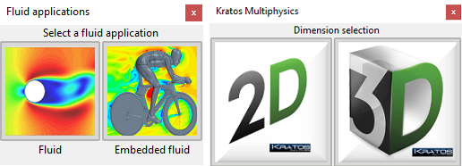
The start data window of the problem type appears. We are going to run a simulation of a 2D fluid flow, so we must click on the Fluid button.

Available applications in the Kratos Market.
In the next window, select again Fluid and 2D,
This will set the kratos tree into a Fluid 2D configuration
Assign fluid material
Materials and properties->Fluid
For applying the fluid material properties double-click on Parts
You can see that a window (like the one shown in the figure) is opened with a data tree containing all the information required for the simulation.
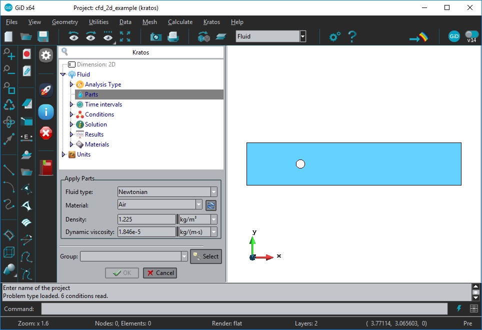
Click in the refresh button next to the material to set the Air values for density and viscosity. Then, click on the Select button and assign the surface. Once selected the surface, click End and Ok.
Run a CFD simulation > Fluid boundaries
Conditions and initial data->Fluid flow
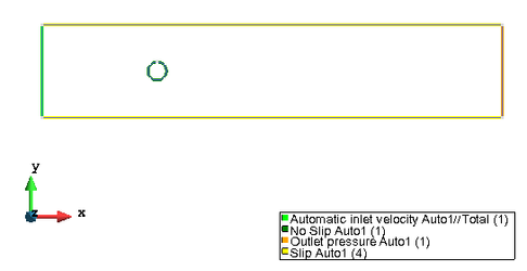
- Unfold the Conditions container of the tree to show the conditions available.
First of all we are going to force the fluid to have null velocity in the 'solid' boundaries of the model, which are the circumference 2D curves (that represent the surfaces of a cylinder considering it as a 3D model)
- Double-click on No slip and a window will appear in the lower part.
- Click on Select, and select the circumference lines.
- Then click End and Ok.
- You'll see that group: No Slip Auto1 has been created and binded to the No Slip condition
Now, we are going to set the lateral walls as Slip
- Double-click on Slip and a window will appear in the lower part.
- Click on Select, and select the top and bottom straight lines of the box.
- Then click End and Ok.
- You'll see that group: Slip Auto1 has been created and binded to the Slip condition
Now we are going to set the conditions for the outlet region (the face of the control volume with maximum X coordinate).
- Double-click on Outlet pressure and a window will appear in the lower part.
- Ensure the options set are
- Not checked → by function
- Not checked → Add hydrostatic contribution
- Value: 0.0 Pa
- Click on Select, and select the line with maximum X coordinate
- Then click End and Ok.
You'll see that group: Outlet pressure has been created and binded to the Outlet pressure condition
It's time to set the conditions for the inlet region (the face of the control volume with minimum X coordinate).
- Double-click on Automatic inlet velocity and a window will appear in the lower part.
- Ensure the options set are
- Not checked → by function
- Value: 3.0 m/s
- Normal direction: Inwards
- Time interval: Total
- Click on Select, and select the surface with minimum X coordinate
- Then click End and Ok.
- You'll see that group: Automatic inlet velocity has been created and binded to the Automatic inlet velocity condition
General data
Now it is time to set the general data for the solver, like solver parameters, etc.
Solution > Parallel configuration
We are going to run this analysis using 8 processors and OpenMP.
Solution > Time parameteres
- End time: 20
- Delta time: 0.1
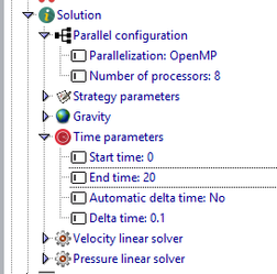
Values for the Solution parameters
Results
Results > General data
- Units used for output frequency: Steps
- Time steps between outputs: 1
Check properties assigned
Clicking on the tree with the right-mouse button, user can check the information assigned to the model, drawing with colors the different conditions, materials, etc... (contextual menu: Draw->Draw groups...)
Tree items with data applied to groups are highlighted in bold characters
Meshing
Make sure you are using a Body fitted mesher in Utilities > Preferences > Meshing >General> Mesh type > Body-fitted.
To mesh the model, click on the menu Mesh > Generate mesh and mesh with mesh size: 0.2
Calculation
You can run the calculation by clicking in the rocket of the left toolbar, or in the menu Calculate > Calculate (F5)
Results
Go to postprocess and check the results.
Extra > CFD 3D
Go back to preprocess and let's create a 3D case.
Go to Files > New. The application selector should appear again. This time we are selecting Fluid > Fluid > 3D. The Kratos team has developed an example to show how to run a 3D cylinder in a Air flow.
Click on the book icon in the left toolbar. ![]()
This will generate the geometry and the tree assignations. You can navigate through the tree and see the assigned values. Save the model, mesh it and run it. (It may take some minutes).
COPYRIGHT © 2022 · GID · CIMNE