Results visualization

Description

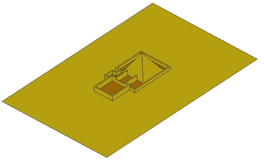
The objective of this course is to do a postprocess analysis of an already calculated fluid simulation around a pyramid building.

In this course, the project pyramid.gid will be used.

Note: the solver used to run this simulations was Tdyn, a fluid dynamic (CFD) simulation environment based on the stabilized Finite Element Method.

Steps followed in this course:

Loading the model
Changing mesh styles
Visualization of results
Creating images

Loading the model

In this course we will use the pyramid project, so the steps to follow are:

Start GiD
Open the pyramid.gid project with: Files->Open, Ctrl-o or clicking on
Switch to postprocess mode: or Files→Postprocess

Note: If you are viewing some popups messages and you want to deactivate them you can do it following these steps:

Select Utilities→Preferences
In General branch choose Normal in the Popup messages option

Changing mesh styles

Menu
Window->View style...

Description

Select Window->View style... using the menu bar or clicking on

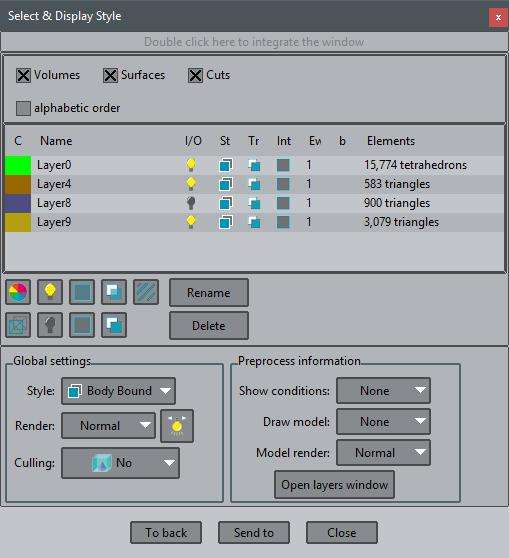
Our model is composed by 4 layers. In order to get a better visualization we will disable the volume layer.

Select the Layer0 layer and switch it off
Select the Layer8 layer and switch it on
Click on the icon in the Tr column or click on the .
Click on Close button

Play a little with the options of these windows, but to continue the tutorial, let a Body Bound style selected for all meshes

Viewing the results

Menu
View results
Window->View results...
Utilities->Preferences->Postprocess branch

Description
Several results had been calculated for several time steps. You can check these results through the View results menu or opening the View Results window.

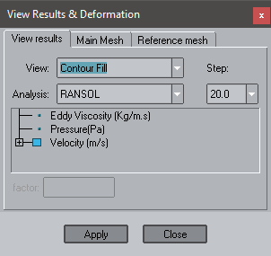
The options related with the results visualization can be changed through the Preferences window, in the Postprocess branch. When you change an option this one turns to red before apply. To apply the changes click on Apply button.

Iso surfaces and animations

Model used
The model pyramid.gid used in this example can be found at Material location.

Menu
View results->Iso Surfaces

Description
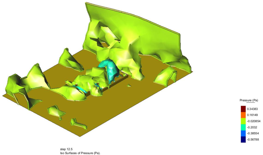
With this result's visualization a surface, or line, is drawn passing through all the points which have the same result's value inside a volume mesh, or surface mesh. To create iso-surfaces there are several options.

From preprocess mode open the model
Switch to postprocess mode
Turn off the Layer0 and Layer8 in order to get a better view
Set as Body Bound the layers style
Select the 12.5 step through View results->Default analysis/step->RANSOL->12.5 or clicking on
Select View results->Iso surfaces->Automatic width->Pressure(Pa) through the menu bar or clicking on

After choosing the result, you are asked for a width. This width is used to create as many isosurfaces as are needed between the Minimum and Maximum defined values (these are included).

Select the default value 0.182341

Several configuration options can be set via the Preferences window.

Menu
Utilities->Preferences->Postprocess->Iso surfaces

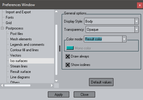
In order to see the inner zones we will set the transparency on the iso surfaces.

For Transparency option select Transparent
Move the model to see the inner zones
For Transparency option select again as Opaque
In order to improve the visualization and to get a more realistic view select View->Render→Smooth

Other interesting options are:

Geometry->Convert->Iso surfaces to sets which consolidates the iso-surface as mesh which can be exported to a file.
Utilities->Preferences->Postprocess->Iso surfaces->Color mode->Contour fill color allows to draw the contour fill of any result over the iso-surface. Select this option and then do a contour fill of any result.
Utilities->Preferences->Postprocess->Iso surfaces->Show isolines this options allows the user to switch iso-lines of surfaces on or off.

Menu
Window->Animate

Description
This window allows the user to animate the current visualized results.

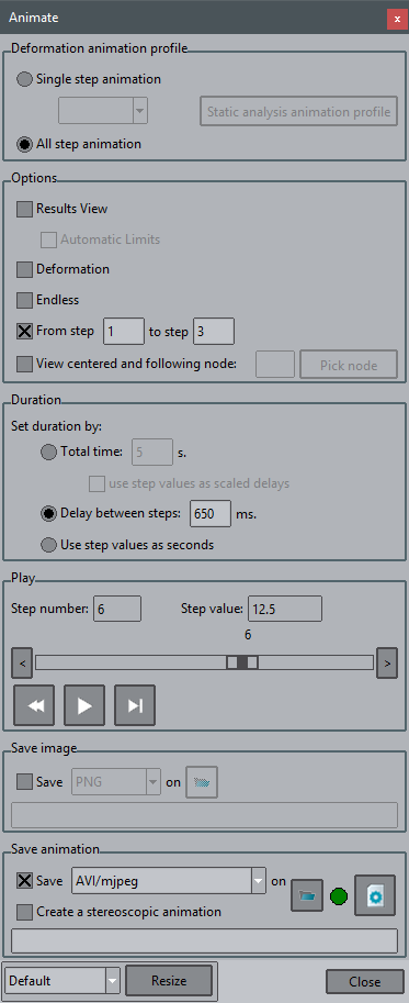
If one result has several steps you can visualize them in an animation. In this case we will use the iso-surfaces result.

Select Window->Animate... or click the icon to open the animation window

Please notice that we have from step 1 to 9. We will do the animation only of some of these steps.

Check the From step option and set 3 to step 9
Select the Delay between steps option and set it to 650 ms. The animation should take around 4 seconds
Try it clicking on the play icon

We will record a video during the animation.

Once the animation is finished check the Save option

You can choose from several video formats.

Select AVI/mjpeg
Please select a folder where the video will be saved clicking on the folder icon or writing the path
Please click on the play button and the recording will begin. This step could take a little bit long. Wait until the red circle turns to green
Close the Animate window

Now we will visualize another result but before we will clear all the results.

Select View results->No results through the menu bar or using the icon

Result surface

Model used
The model pyramid.gid used in this example can be found at Material location.

Menu
View results->Result surface

Description
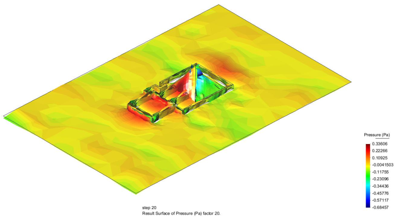
This option uses a result component, or a scalar value, and draws a 3D surface above the mesh following the normals of this mesh.

From preprocess mode open the model
Switch to postprocess mode
In order to get a better view turn off the Layer0 and Layer8 layers
Select View->Render->Smooth
Select View results->Result surface-> Pressure (Pa). A surface will be drawn which results from moving the nodes along its smoothed normal according to the results value for this node
Enter 20 as factor in the command line
Due we have positive and negative values please set as Boundaries the layers style. Now all the result surface can be seen easily
You can change several options in the Preferences window
Select Utilities->Preferences->Postprocess->Result surface->Show elevations->None
Select Utilities->Preferences->Postprocess->Result surface->Draw contour fill. With this last option the surface is colored according to the pressure value
Click on Apply button
Play with the other options as you will
Click on Close button
Select View results->No results through the menu bar or using the icon

Contour fill, cuts and limits

Model used
The model pyramid.gid used in this example can be found at Material location.

Contour fill
Menu
View results->Contour Fill

Description
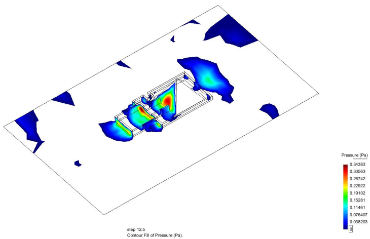
This option allows the visualization of coloured zones, in which a scalar variable or a component of a vector varies between two defined values.

From preprocess mode open the model
Switch to postprocess mode
In order to get a better view turn off the Layer0 and Layer8 layers
Set as Body Bound the layers style
Select View->Render->Normal
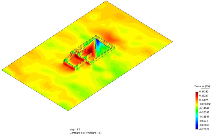
Please select View results->Contour fill->Pressure (Pa) through the menu bar, or clicking on or using the Window->View results... window

GiD can use as many colours as permitted by the graphical capabilities of the computer. The number of colours can be set through Utilities->Preferences->Postprocess->Contour fill and lines->By number of colors. A menu of the variables to be represented will be shown, and the one that is chosen will be displayed using the default analysis and step selected.
In the model the pressure has been calculated. We can visualize the result for each step in a contour fill.
You can choose the step that you want to view through the View results window or clicking on

Select the step 12.5

Several configuration options can be set via the Preferences window.

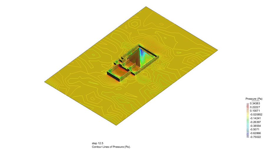
NOTE: Another similar result visualization is Contour lines but in this case the iso-lines of a certain nodal variable are drawn. In this case, each color ties the points with the same value of the variable chosen.

Menu
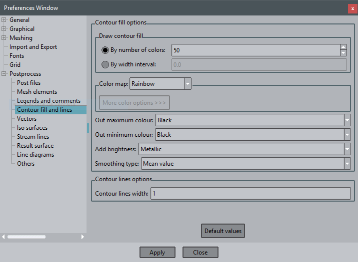
Utilities->Preferences->Postprocess->Contour fill and lines

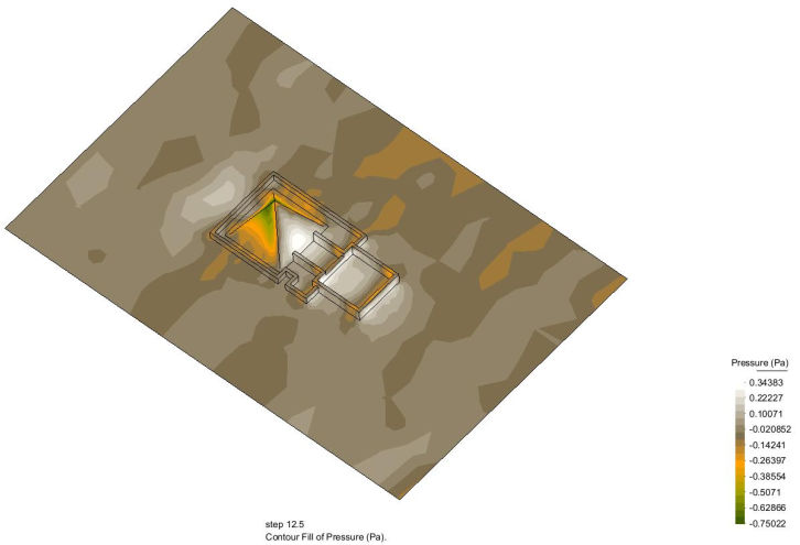
You can change the color scale in other to get a more comfortable view. You can select several predefined color scales. The default scale is Rainbow, starting from blue (minimum) through green and yellow, to red (maximum).

For Color map option select Terrain

You can also set your own scale.

For Color map option select User defined
Select the button More color options to open a window.In this window you can change the number of different colors used in the scale. If you need more accuracy you can increase this number, or decrease it for a higher contrast.
Change the number of colors to 20
Click on Apply button
Click on Close button
Click on Apply button of the preferences window

Cuts
Menu
Geometry
In order to view the inner zone we will do several cuts along the model.

We want to cut the inner volume in order to see the pressure in the air.
First of all we have to make visible the volume.

Select Window->View style...
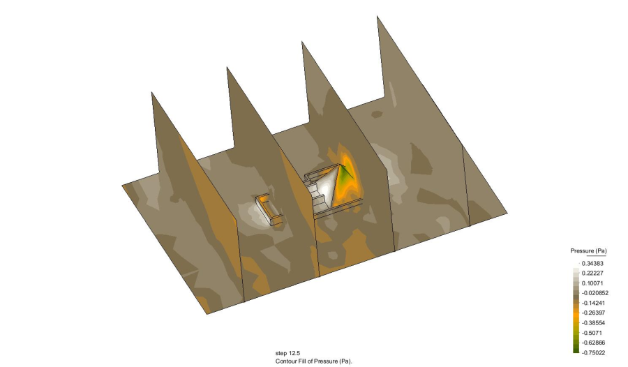
Select Layer0 and make it visible clicking on theicon
Select Geometry->Cut plane->Succesion through the menu bar or clicking on and then

With the succession option you specify a line which will be used as axis to create cut planes orthogonal to this axis.

NOTE: after clicking the first point, you can press the Alt key to snap the dynamic line to the screen horizontal, vertical or 45º diagonals.
The number of planes is also asked for.

The axis is defined by two points, please write the first one in the command line 30 200 0
You are asked for the second point, introduce 30 -100 0
Choose 4 cuts. You should obtain 4 parallel planes to Y axis.
Select Window->View style... You can see that several layers had appeared a prefix like CutX. These names can always be changed through this window
Set off the Layer0 again through the View style window. You can rotate the model in order to see the contour fill result on the cut planes.
In the same window select all the CutX and click on Delete button in order to delete all the cuts.
Select Yes
In order to reset the default options for the contour fill, go to Utilities->Preferences->Postprocess->Contour fill and lines
Click on Default values button
Click on Apply button

Define limits
You can set the limit values for the contour fill. In our case we only want to see the positive values. In order to do this we will set the minimum value to 0.

. Select Utilities->Set contour limits->Define limits... through the menu bar or clicking on

Choosing the first option the Contour Limits window appears. With this window you can set the minimum/maximum value that Contour Fill should use.

Check the Min checkbox
Change the value to 0
Click on the Apply button
Click on the Close button

Outliers will be drawn in the colour defined in the Out Min Colour option. In order to view it better we will change this color to transparent.

Select Utilities->Preferences->Postprocess->Contour fill and lines->Out minimum color->Transparent
Click on Apply button
Select Utilities->Set contour limits->Reset limits
Select View results->No results

Combined results

Model used
The model pyramid.gid used in this example can be found at Material location.

Menu
Window->Several results...

Description
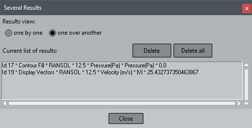
Through this window you can select several results in order to visualize them at the same time. From this window you can also delete the undesired results visualizations.

From preprocess mode open the model
Switch to postprocess mode
In order to get a better view turn on all the layers except Layer8
Set Layer0 transparent
Set as Body Bound the layers style

In order to see the inner vectors first we will do a cut through the volume. We want a cut parallel to the XY plane and near to the pyramid base.

Select View->Rotate->Plane YZ to get a proper view to make de cut
Select Geometry->Cut plane->2 points
Select 2 points by your own near the pyramid
Press ESC to leave the cut function
Turn off the Layer0
Change the cut layers style to Boundaries
Select Window->Several results...
In this window select one over another. With this option GiD is told to visualize one result over another
Select View results->Default analysis/step->Ransol->12.5
Select View Results->Contour fill->Pressure
Select View results->Display vectors->Velocity (m/s)->|V|
Select Utilities->Preferences->Postprocess->Vectors->Color mode and select By modules and click on Apply button
Select View results->No results
Delete the created cuts

Show min max

Model used
The model pyramid.gid used in this example can be found at Material location.

Menu
View results->Show Min Max

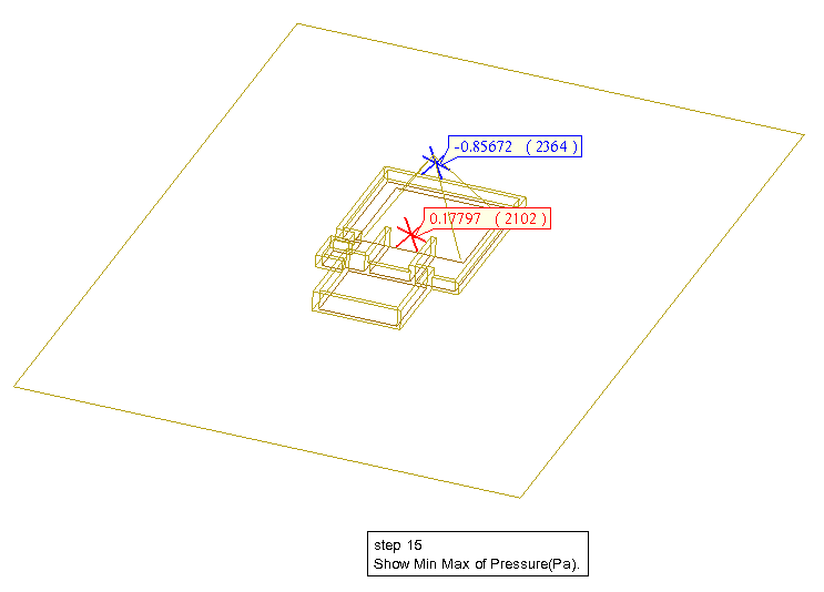
Description
With this option you can see the minimum and maximum value of the chosen result in the chosen analysis step. In our case we will choose the Vy component of velocity result for the first analysis step.

From preprocess mode open the model
Switch to postprocess mode
Turn off the Layer0 and Layer8 in order to get a better view
Change the style to Boundaries for all the layers
Select View results->Default analysis/step->RANSOL->15 through the menu bar or clicking on
Select View results->Show min max->Show both->Pressure (Pa) through the menu bar or clicking on . The label shows the node number and the value of the result
Select View results->No results

Display Vectors

Model used
The model pyramid.gid used in this example can be found at Material location.

Menu
View results->Display Vectors

Description
With this display option the nodal vectors of the chosen result are shown.

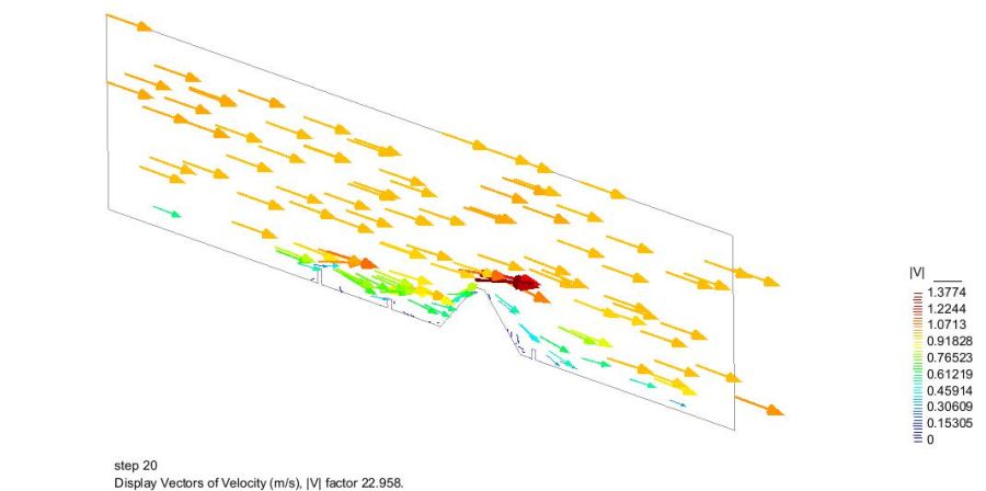
We want to display the vectors of velocity in a cut.

From preprocess mode open the model
Switch to postprocess mode
Turn on all the layers except Layer8
Set Layer0 transparent
Select View results->Default analysis/step->RANSOL->20 throught the menu bar or clicking on

In order to see the inner vectors first we will do a cut through the volume. We want a cut parallel to the YZ plane and near to the pyramid center

Select View->Rotate->Plane XY (Original) to get a proper view to make de cut
Select Geometry->Cut plane->2 points
Select 2 points by your own or enter the following coordinates in the command line. 30 200 and 30 -100
Press ESC to leave the cut function
Turn off all the layers except the ones with name CutX in order to only see the cut
For all the cut layers change the style to Boundaries
Select View results->Display vectors->Velocity (m/s)->|V|

Menu
Utilities->Preferences->Postprocess→Vectors

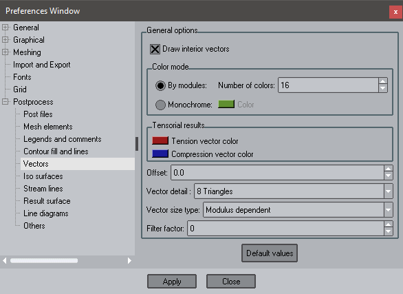
For Color Mode option select By modules in order to see the vectors by colors depending on their value
The option Number of colors turns on. Enter 50 and click on Apply to get more accuracy
For Filter factor option, enter 5 and click Apply. This option changes the number of displayed vectors
Click on Close button
Delete the layers with name CutX
Select View results->No results

Stream lines

Model used
The model pyramid.gid used in this example can be found at Material location.

Menu
View results->Stream Lines

Description
With this option you can display a stream line, or in fluid dynamics, a particle tracing, in a vector field.

From preprocess mode open the model
Switch to postprocess mode
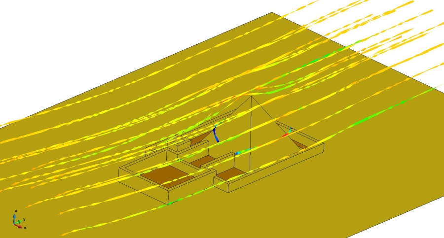
Turn on all the layers except Layer8
Set Layer0 transparent
Set as Body Bound the layers style

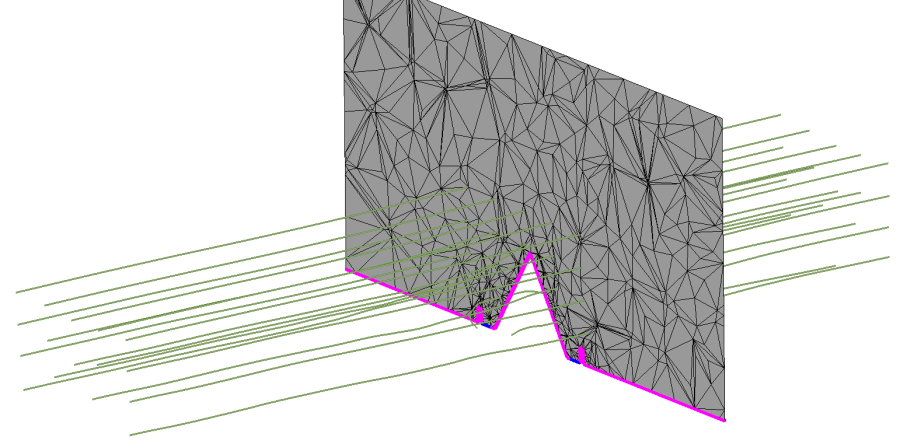
We want to create some stream lines near the pyramid center in order to plot the velocity result near it. So we will make a cut near the center and we will select there the points where we want to plot the stream lines. We want a cut parallel to the XZ plane and near to the pyramid center.

Select View->Rotate->Plane XY (Original) to get a proper view to make de cut
Select Geometry->Cut plane->2 points
Select 2 points by your own or enter the following coordinates in the command line. -70 78 and 130 78
Press ESC to leave the cut function
For each cut created change the style to Body Lines
To get a better view set off all the layers except the ones with name CutX
Select View->Rotate->Plane XZ
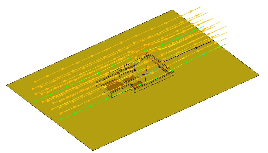
Select View results->Stream lines->In a quad->Velocity (m/s) through the menu bar

With this option you can define a quadrilateral area which will be used to create a N x M matrix of points. These points will be the start for the stream lines.
We want to create several stream lines around the pyramid.

Note: This action could also be done clicking on in the icon bar. In this case we have to select the way to define the start point through the mouse menu. In this case select Contextual->In A Quad.

From the mouse menu (right button click) select Contextual->Join Ctrl-a
Define a quadrilateral area near the pyramid shape clicking on 4 mesh points
You are asked for the number of points in the quad. Enter 5,5 and click Ok

The stream lines are created.

Click the middle mouse button or press the ESC key in order to finish the operation
Turn off the cuts layers and set on the layers Layer4 and Layer9

Menu
Utilities->Preferences->Postprocess->Stream lines

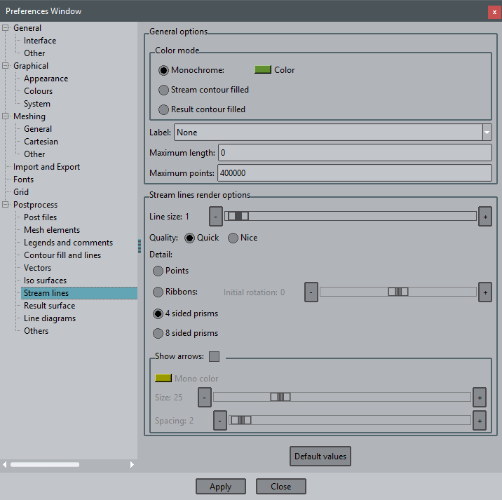
Select Utilities->Preferences->Postprocess->Stream lines
In color mode section, select Stream contour filled option. The stream lines will be drawn with the colors used in the velocity contour fill
In render options section,change the Line size to 2
And select Quality->Nice option in order to draw the stream lines with triangles
And Detail->Ribbons. With this option the streams show the swirl of the velocity field
Click on Apply
Change the Detail to 4 sided prism again
Check the Show arrows option
Set 20 for the Size option
Set 20 for the Spacing option
Clilck Apply
Click on Close button
Select View results->Delete->Stream lines->All
Delete the created cuts

It's also possible to save the stream lines for next sessions.

Select Files->Export->Post information->Stream lines...
Choose the location where you want to save them and click on Save

Then you can import them with Files->Import->Stream lines...

Graphs

Model used
The model pyramid.gid used in this example can be found at Material location.

Menu
View results->Graphs

Description
From this menu several graphs types can be created, we will try some of them. Graphs are supported for results defined over nodes.
Graphs are organized into graph sets in order to ease the management. Each set shares the same units for each axis.
When a graph is created is placed in the current graphset if the units are the same, otherwise a new graphset is created.
In order to work with graphs we will use the 'graphs window'.

From preprocess mode open the model
Switch to postprocess mode
Turn on all the layers except the Layer8 through the View style window
Change the mesh style to boundaries for all the layers

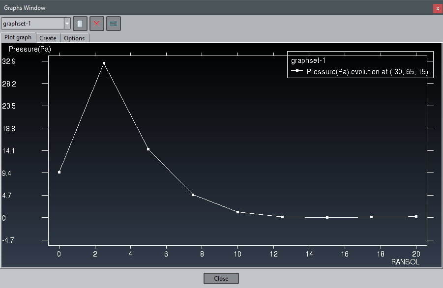
The Point evolution graph displays a graph of the evolution of the selected result along all the steps, of the default analysis, for the selected nodes.

Select View results->Graphs->Point evolution->Pressure (Pa)
Write 30 65 15 in the command line in order to specify the point
Affter pressing the Escape key, or the middle mouse button, the graph will be shown in a separate window:

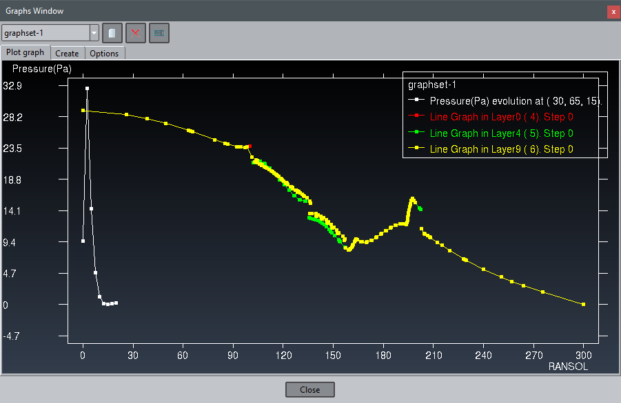
The graph is created in the graphset-1. We will create another graph in the same graph set.

The Line graph displays a graph defined by the line connecting two selected nodes of surfaces or volumes, or any arbitrary points on any projectable surface and in any position.

Select View results->Default analysis/step->RANSOL->0
Select View results->Graphs->Line graph->Pressure(Pa)
Write 30 -100 0 in the command line in order to specify the initial point
Write 30 200 0 in the command line in order to specify the final point

Now both graphs are shown in the same graph set:

Note: probably it is a bad idea to represent both kind of graphs in the same graphset x-y space, because the x axis for the 'Point evolution' represents the time step (e.g. seconds) and for the 'Line graphs' represent a spatial distance (e.g. meters).

We will rename the graph set.

In the top part of the window click the icon
A window will appear asking for a new name. Enter 'Pressure', for example

We will create a new graph set.

In the top part of the window click the icon

A new graph set is created with default name 'graphset-1'. When a new graph set is created becomes the current one. We can see that there are no graphs on this new graph set.
It's also possible to create graphs from the graph window.

Go to Create tab and select Point Evolution int View option
In Y Axis list double click Velocity (m/s)->|V|
Write 30 65 15 in the command line in order to specify the point
Press Escape to finish the graph.

We can manage graphs and graphs sets in the Options panel. Depending if we are selecting a graph set or a graph in the tree we will see different options in the tab.

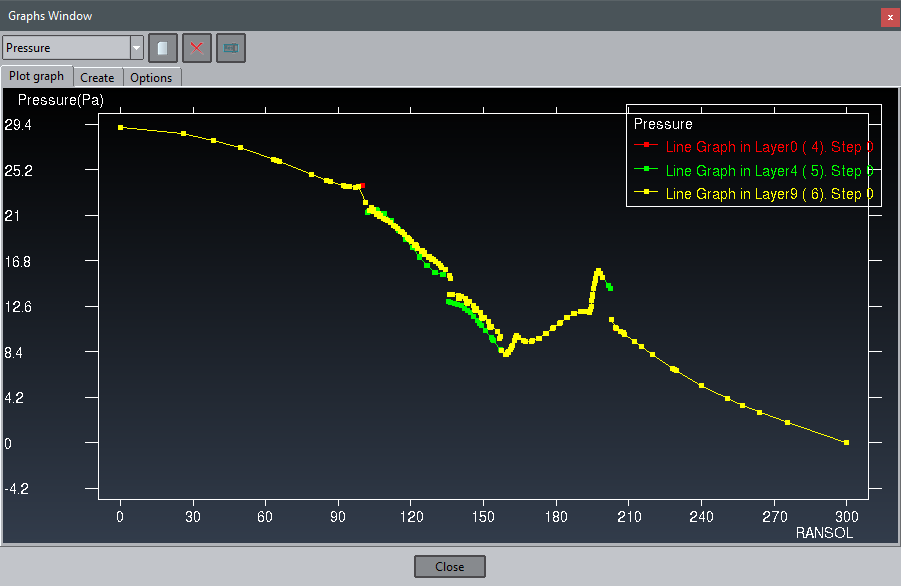
Go to the Options panel, select the 'Pressure (Pa) evolution at (30, 65, 15)' graph and delete it pressing the button with the red cross.
A confirmation window appears. Click Yes.

Please notice that the current graph set have been changed to 'Pressure'. Now the Plot graph panel will show only three graphs:

The graph size is re-adapted. We will change several style options of a graph.

Double click in any point of one graph and we will access to the Options tab
Choose Line in the Style option
Set to red the Color option. You can do it writing #ff0000 (hexadecimal values of red, green and blue color components) or selecting the white color clicking on the right color window
Set to 4.0 the Line width
Click on Apply button

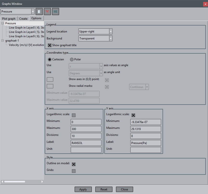
Graph sets options can be managed selecting the set in the tree.

Select 'Pressure' branch. The options will change.
For instance mark 'Logarithmic scale' option in Y axis.
Click on Apply button

We can export the graph information in order to open it later with GiD.

Select Files->Export->Graph->All graphsets. You are asked for the location where to save the .grf file
Choose the location

Now you can import the graphs selecting Files->Import->Graph...